Code
box::use(
    dplyr[...],
    tidyr[...],
    ggplot2[...],
    gghdx[...],
    cumulus[...],
    purrr[...],
    tibble[tibble]
)

gghdx()This chapter compares the in-sample performance metrics between the 2025 and 2026 trigger models.
Both models use different validation approaches:
These LOOCV approaches test different things and aren’t directly comparable. For a fair comparison, we use in-sample metrics for both.
| Aspect | 2025 | 2026 |
|---|---|---|
| Approach | Weight grid search | Ridge regression |
| Spatial unit | Per province (3 models) | Merged 5-province area (1 model) |
| Weight selection | Best F1 from ~200k combinations | Regularized coefficients |
box::use(
dplyr[...],
tidyr[...],
ggplot2[...],
gghdx[...],
cumulus[...],
purrr[...],
tibble[tibble]
)
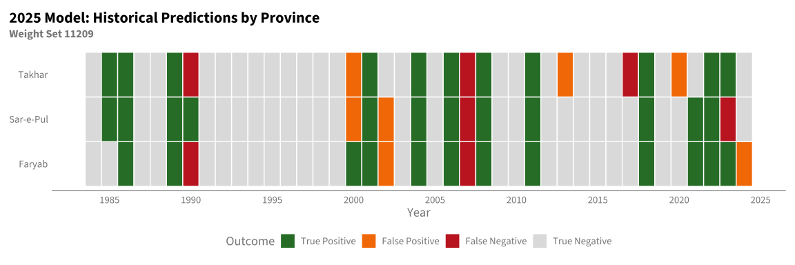
gghdx()The 2025 model used weight set 11209, selected from an exhaustive grid search.
# Load the 2025 weight set time series
df_2025 <- blob_read(
    name = "ds-aa-afg-drought/trigger_timeseries/cdi_wt_id_11209.parquet",
    container = "projects"
)# Calculate F1 per province
# zscore_flag = CDI exceeds threshold (predicted drought)
# zscore_asi_Jun_flag = ASI exceeds threshold (actual drought)
df_2025_metrics <- df_2025 |>
group_by(adm1_name) |>
summarise(
n_years = n(),
tp = sum(zscore_flag & zscore_asi_Jun_flag, na.rm = TRUE),
fp = sum(zscore_flag & !zscore_asi_Jun_flag, na.rm = TRUE),
fn = sum(!zscore_flag & zscore_asi_Jun_flag, na.rm = TRUE),
tn = sum(!zscore_flag & !zscore_asi_Jun_flag, na.rm = TRUE),
.groups = "drop"
) |>
mutate(
precision = tp / (tp + fp),
recall = tp / (tp + fn),
f1 = 2 * tp / (2 * tp + fp + fn)
)
df_2025_metrics |>
select(adm1_name, n_years, tp, fp, fn, precision, recall, f1) |>
knitr::kable(
digits = 3,
caption = "2025 Model: In-Sample Performance by Province (Weight Set 11209)",
col.names = c("Province", "N Years", "TP", "FP", "FN", "Precision", "Recall", "F1")
)| Province | N Years | TP | FP | FN | Precision | Recall | F1 |
|---|---|---|---|---|---|---|---|
| Faryab | 41 | 12 | 2 | 2 | 0.857 | 0.857 | 0.857 |
| Sar-e-Pul | 41 | 12 | 2 | 2 | 0.857 | 0.857 | 0.857 |
| Takhar | 41 | 11 | 3 | 3 | 0.786 | 0.786 | 0.786 |
df_2025_avg <- df_2025_metrics |>
    summarise(
        across(c(precision, recall, f1), mean, na.rm = TRUE)
    ) |>
    mutate(model = "2025 (avg over provinces)")

df_2025_avg |>
    select(precision, recall, f1) |>
    knitr::kable(
        digits = 3,
        caption = "2025 Model: Average In-Sample Performance"
)| precision | recall | f1 |
|---|---|---|
| 0.833 | 0.833 | 0.833 |
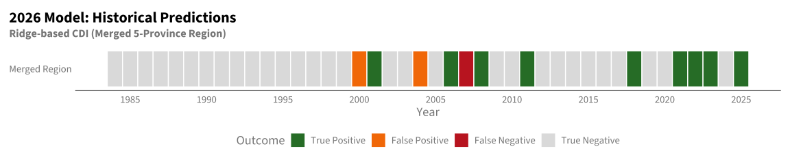
The 2026 model uses ridge regression on a merged 5-province area. In-sample metrics from Chapter 12:
df_2026 <- tibble(
    model = "2026 (merged region)",
    precision = 0.818,
    recall = 0.900,
    f1 = 0.857
)

df_2026 |>
    select(precision, recall, f1) |>
    knitr::kable(
        digits = 3,
        caption = "2026 Model: In-Sample Performance"
)| precision | recall | f1 |
|---|---|---|
| 0.818 | 0.9 | 0.857 |
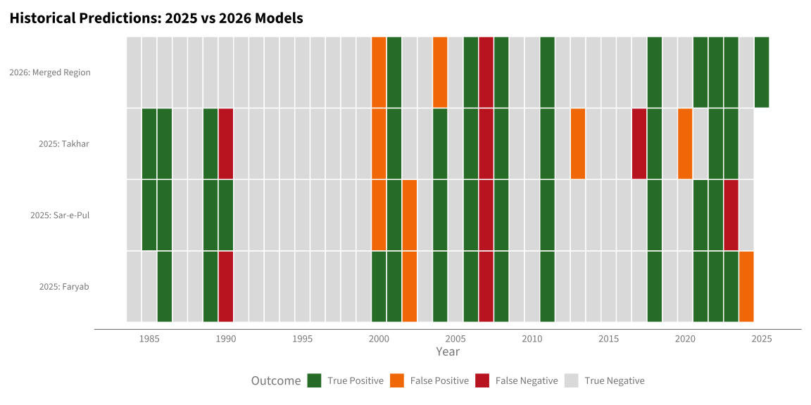
To visualize how each model performs year-by-year, we create heatmaps showing predicted vs actual drought outcomes.
# Load 2026 feature set and compute CDI predictions
df_2026_raw <- blob_read(
    name = "ds-aa-afg-drought/processed/vector/2026_april_pub_feature_set_v1.parquet",
    container = "projects"
)

# CDI weights from Chapter 12 (ridge regression)
# vhi: ~29%, mixed_fcast_obsv: ~24%, snow_cover: ~19%, asi: ~16%, soil_water: ~12%
CDI_THRESHOLD <- 0.503  # F1-optimized threshold from Chapter 12

# Calculate CDI for 2026 model
df_2026_preds <- df_2026_raw |>
    filter(!is.na(outcome_asi_zscore)) |>
    mutate(
        # Calculate CDI as weighted sum
        CDI = vhi * 0.291 + mixed_fcast_obsv * 0.243 + snow_cover * 0.188 +
              asi * 0.156 + volumetric_soil_water_1m * 0.122,
        year = pub_year
    ) |>
    # Calculate empirical RP for outcome (ASI) - defines "actual" drought
    arrange(desc(outcome_asi_zscore)) |>
    mutate(
        rank_asi = row_number(),
        rp_asi = (n() + 1) / rank_asi,
        actual = rp_asi >= 4  # ASI RP >= 4 = drought year
    ) |>
    # Prediction based on CDI threshold (not RP)
    mutate(
        predicted = CDI >= CDI_THRESHOLD  # F1-optimized threshold from Ch 12
    ) |>
    select(year, CDI, outcome_asi_zscore, predicted, actual) |>
arrange(year)# Prepare 2025 data for heatmap
df_2025_heatmap <- df_2025 |>
mutate(
year = as.numeric(format(as.Date(yr_season), "%Y")),
predicted = zscore_flag,
actual = zscore_asi_Jun_flag,
outcome = case_when(
predicted & actual ~ "TP",
predicted & !actual ~ "FP",
!predicted & actual ~ "FN",
TRUE ~ "TN"
)
) |>
select(year, adm1_name, predicted, actual, outcome)
# Prepare 2026 data for heatmap
df_2026_heatmap <- df_2026_preds |>
mutate(
adm1_name = "Merged Region",
outcome = case_when(
predicted & actual ~ "TP",
predicted & !actual ~ "FP",
!predicted & actual ~ "FN",
TRUE ~ "TN"
)
) |>
select(year, adm1_name, predicted, actual, outcome)outcome_colors <- c(
"TP" = "#2E7D32", # Green - correct positive
"TN" = "#E0E0E0", # Light gray - correct negative
"FP" = "#F57C00", # Orange - false alarm
"FN" = "#C62828" # Red - missed
)
df_2025_heatmap |>
mutate(
outcome = factor(outcome, levels = c("TP", "FP", "FN", "TN")),
adm1_name = factor(adm1_name, levels = c("Faryab", "Sar-e-Pul", "Takhar"))
) |>
ggplot(aes(x = year, y = adm1_name, fill = outcome)) +
geom_tile(color = "white", linewidth = 0.5) +
scale_fill_manual(
values = outcome_colors,
labels = c("TP" = "True Positive", "TN" = "True Negative",
"FP" = "False Positive", "FN" = "False Negative")
) +
scale_x_continuous(breaks = seq(1985, 2025, by = 5)) +
labs(
title = "2025 Model: Historical Predictions by Province",
subtitle = "Weight Set 11209",
x = "Year",
y = NULL,
fill = "Outcome"
) +
theme(
legend.position = "bottom",
panel.grid = element_blank()
)
df_2026_heatmap |>
    mutate(outcome = factor(outcome, levels = c("TP", "FP", "FN", "TN"))) |>
    ggplot(aes(x = year, y = adm1_name, fill = outcome)) +
    geom_tile(color = "white", linewidth = 0.5) +
    scale_fill_manual(
        values = outcome_colors,
        labels = c("TP" = "True Positive", "TN" = "True Negative",
                   "FP" = "False Positive", "FN" = "False Negative")
    ) +
    scale_x_continuous(breaks = seq(1985, 2025, by = 5)) +
    labs(
        title = "2026 Model: Historical Predictions",
        subtitle = "Ridge-based CDI (Merged 5-Province Region)",
        x = "Year",
        y = NULL,
        fill = "Outcome"
    ) +
    theme(
        legend.position = "bottom",
        panel.grid = element_blank()
    )
# Combine both datasets
df_combined_heatmap <- bind_rows(
    df_2025_heatmap |> mutate(model = "2025"),
    df_2026_heatmap |> mutate(model = "2026")
) |>
    mutate(
        panel = paste0(model, ": ", adm1_name),
        panel = factor(panel, levels = c(
            "2025: Faryab", "2025: Sar-e-Pul", "2025: Takhar",
            "2026: Merged Region"
        )),
        outcome = factor(outcome, levels = c("TP", "FP", "FN", "TN"))
    )

df_combined_heatmap |>
    ggplot(aes(x = year, y = panel, fill = outcome)) +
    geom_tile(color = "white", linewidth = 0.5) +
    scale_fill_manual(
        values = outcome_colors,
        labels = c("TP" = "True Positive", "TN" = "True Negative",
                   "FP" = "False Positive", "FN" = "False Negative")
    ) +
    scale_x_continuous(breaks = seq(1985, 2025, by = 5)) +
    labs(
        title = "Historical Predictions: 2025 vs 2026 Models",
        x = "Year",
        y = NULL,
        fill = "Outcome"
    ) +
    theme(
        legend.position = "bottom",
        panel.grid = element_blank(),
        axis.text.y = element_text(size = 10)
    )
# Compare 2025 (majority vote across provinces) with 2026
df_2025_majority <- df_2025_heatmap |>
    group_by(year) |>
    summarise(
        predicted_2025 = sum(predicted) >= 2,  # majority vote
        actual_2025 = sum(actual) >= 2,
        .groups = "drop"
    )

df_comparison_years <- df_2025_majority |>
    inner_join(
        df_2026_heatmap |> select(year, predicted_2026 = predicted, actual_2026 = actual),
        by = "year"
    ) |>
    mutate(
        models_agree = predicted_2025 == predicted_2026,
        outcome_2025 = case_when(
            predicted_2025 & actual_2025 ~ "TP",
            predicted_2025 & !actual_2025 ~ "FP",
            !predicted_2025 & actual_2025 ~ "FN",
            TRUE ~ "TN"
        ),
        outcome_2026 = case_when(
            predicted_2026 & actual_2026 ~ "TP",
            predicted_2026 & !actual_2026 ~ "FP",
            !predicted_2026 & actual_2026 ~ "FN",
            TRUE ~ "TN"
        )
    )

# Show years where models disagree
df_comparison_years |>
    filter(!models_agree) |>
    select(year, outcome_2025, outcome_2026) |>
    knitr::kable(
        caption = "Years Where 2025 (Majority Vote) and 2026 Models Disagree",
        col.names = c("Year", "2025 Outcome", "2026 Outcome")
)| Year | 2025 Outcome | 2026 Outcome |
|---|---|---|
| 1985 | TP | TN |
| 1986 | TP | TN |
| 1989 | TP | TN |
| 2002 | FP | TN |
df_comparison <- bind_rows(
    df_2025_metrics |>
        select(precision, recall, f1) |>
        mutate(model = paste0("2025 ", df_2025_metrics$adm1_name)),
    df_2025_avg |> select(model, precision, recall, f1),
    df_2026
) |>
    select(model, precision, recall, f1)

df_comparison |>
    knitr::kable(
        digits = 3,
        caption = "In-Sample Performance Comparison: 2025 vs 2026",
        col.names = c("Model", "Precision", "Recall", "F1")
)| Model | Precision | Recall | F1 |
|---|---|---|---|
| 2025 Faryab | 0.857 | 0.857 | 0.857 |
| 2025 Sar-e-Pul | 0.857 | 0.857 | 0.857 |
| 2025 Takhar | 0.786 | 0.786 | 0.786 |
| 2025 (avg over provinces) | 0.833 | 0.833 | 0.833 |
| 2026 (merged region) | 0.818 | 0.900 | 0.857 |
df_comparison |>
    mutate(
        model = factor(model, levels = rev(model)),
        model_type = case_when(
            grepl("2025", model) & !grepl("avg", model) ~ "2025 (by province)",
            grepl("2025", model) ~ "2025 (average)",
            TRUE ~ "2026"
        )
    ) |>
    ggplot(aes(x = f1, y = model, fill = model_type)) +
    geom_col(width = 0.7) +
    geom_text(aes(label = round(f1, 3)), hjust = -0.1, size = 3.5) +
    scale_x_continuous(limits = c(0, 1), expand = c(0, 0.05)) +
    scale_fill_manual(values = c(
        "2025 (by province)" = "steelblue",
        "2025 (average)" = "darkblue",
        "2026" = "tomato"
    )) +
    labs(
        title = "In-Sample F1 Score Comparison: 2025 vs 2026",
        x = "F1 Score",
        y = NULL,
        fill = "Model"
    ) +
    theme(legend.position = "bottom")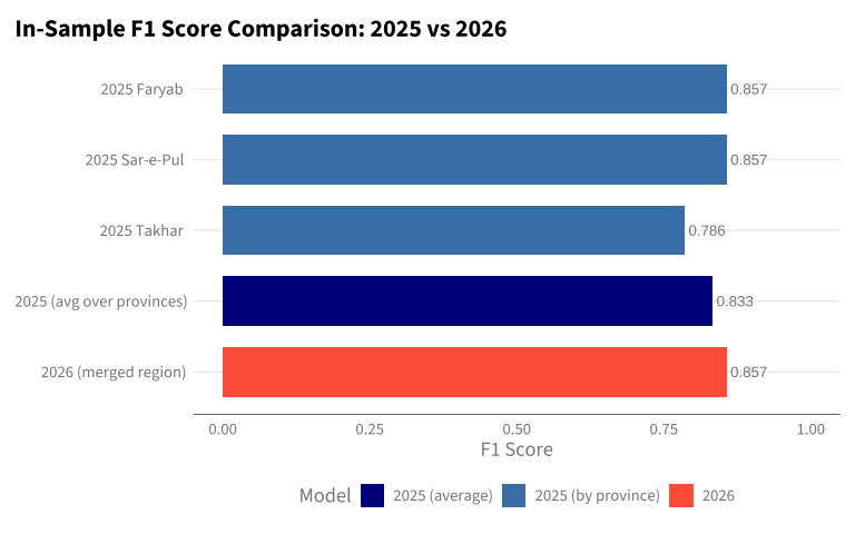
tibble(
    Metric = c("F1 Score", "Precision", "Recall", "Spatial Unit", "N Years"),
    `2025 Model` = c(
        round(df_2025_avg$f1, 3),
        round(df_2025_avg$precision, 3),
        round(df_2025_avg$recall, 3),
        "Per province (avg of 3)",
        "41 per province"
    ),
    `2026 Model` = c(
        "0.857",
        "0.818",
        "0.900",
        "Merged 5-province",
        "42"
    )
) |>
knitr::kable(caption = "Summary: In-Sample Performance Comparison")| Metric | 2025 Model | 2026 Model |
|---|---|---|
| F1 Score | 0.833 | 0.857 |
| Precision | 0.833 | 0.818 |
| Recall | 0.833 | 0.900 |
| Spatial Unit | Per province (avg of 3) | Merged 5-province |
| N Years | 41 per province | 42 |
In-sample comparison (both models evaluated on training data):
| Model | F1 | Precision | Recall |
|---|---|---|---|
| 2025 (avg) | 0.833 | 0.833 | 0.833 |
| 2026 | 0.857 | 0.818 | 0.900 |
The 2026 model shows slightly higher F1 (0.857 vs 0.833) with notably higher recall (0.900 vs 0.833).
Caveats: