10  Pre-Season Trigger - Allocation Model Options & Joint RPs

10.1 Intro

This document explores the thresholds and implied joint return periods based on AOI and months monitored (number of possible activation moments)

Outputs being copied into this slide deck

aoi_adm1 <- c(
    "Takhar",
    "Badakhshan",
    # "Badghis",
    "Sar-e-Pul",
    "Faryab"
)

SEASON_OF_INTEREST <- c(3, 4, 5)
LATEST_SEASON_PREDICTABLE <- c(3, 4)
RP_THRESHOLD <- c(3, 4, 5)

box::use(
    loaders = .. / R / load_funcs,
    seas5 = .. / R / seas5_utils,
    .. / R / blob_connect,
    .. / R / utils[download_fieldmaps_sf, load_aoi_names],
    .. / R / utils,
    .. / R / pg
)

box::use(
    dplyr[...],
    forcats[...],
    ggplot2[...],
    gt[...],
    gghdx[...],
    cumulus,
    DBI,
    RPostgres,
    janitor[clean_names],
    lubridate[...],
    purrr[...],
    readr,
    scales,
    stats,
    stringr[...],
    tidyr[...],
    glue[...]
)
gghdx()

lgdf <- cumulus$download_fieldmaps_sf(iso3 = "AFG", layer = list("afg_adm0", "afg_adm1", "afg_adm2"))

df_seas5_adm2 <- seas5$load_seas5_historical_weighted(weight_set = "WT_ADM2")
df_seas5_adm1 <- seas5$load_seas5_historical_weighted(weight_set = "WT_ADM1")

df_seas5_adm1_mam <- seas5$aggregate_forecast(
    df_seas5_adm1,
    valid_months = c(3, 4, 5),
    by = c(
        "iso3",
        "pcode",
        "adm1_name",
        "n_upsampled_pixels", # keep in for flexible weighting
        "issued_date"
    )
) |>
    mutate(
        pub_mo = month(issued_date, label = T, abbr = T)
    )
df_seas5_adm2_mam <- seas5$aggregate_forecast(
    df_seas5_adm2,
    valid_months = c(3, 4, 5),
    by = c(
        "iso3",
        "pcode",
        "adm1_name",
        "adm1_pcode",
        "adm2_name",
        "n_upsampled_pixels",
        "issued_date"
    )
)

# custom grouped aggregations
df_seas5_mam_no_wakhan <- df_seas5_adm2_mam |>
    group_by(valid_month_label,
        iso3,
        adm1_name,
        adm1_pcode,
        issued_date,
        pub_mo = month(issued_date, label = T, abbr = T),
        leadtime
    ) |>
    summarise(
        mm = weighted.mean(mm, w = n_upsampled_pixels),
        .groups = "drop"
    ) |>
    rename(
        pcode = adm1_pcode
    )

# 1 - single AOI - Badakshan removed
df_seas_mam_aoi1 <- df_seas5_adm1_mam |>
    filter(adm1_name != "Badakhshan") |>
    group_by(valid_month_label, iso3, issued_date, pub_mo = month(issued_date, label = T, abbr = T), leadtime) |>
    summarise(
        mm = weighted.mean(mm, w = n_upsampled_pixels),
        .groups = "drop"
    )

# 2 AOIs - North Central/North East
df_seas5_region_mam <- df_seas5_adm1_mam |>
    mutate(
        region = ifelse(adm1_name %in% c("Faryab", "Sar-e-Pul"), "North Central", "North East")
    ) |>
    group_by(valid_month_label, iso3, region, issued_date, pub_mo = month(issued_date, label = T, abbr = T), leadtime) |>
    summarise(
        mm = weighted.mean(mm, w = n_upsampled_pixels),
        .groups = "drop"
    )

box::reload(seas5)

threshold_sets <- c("ADM1_AOI4", "ADM1_AOI4_NO_WAKHAN", "ADM1_AOI2", "ADM1_AOI1")
threshold_sets <- set_names(threshold_sets, threshold_sets) # name em

ldf_thresholds <- map(threshold_sets, ~ seas5$load_seas5_threshold_tables(.x))



df_sea5_mam_aoi4_classified <- df_seas5_adm1_mam |>
    left_join(
        # attach 3 levels of thresholds
        filter(ldf_thresholds$ADM1_AOI4, rp %in% c(3, 4, 5)),
        relationship = "many-to-many",
        by = c("iso3", "pcode", "adm1_name", "pub_mo", "leadtime")
    ) |>
    mutate(
        flag = mm < rv
    )

df_seas5_mam_aoi4_no_wakhan_classified <- df_seas5_mam_no_wakhan |>
    left_join(
        ldf_thresholds$ADM1_AOI4_NO_WAKHAN |>
            filter(
                rp %in% c(3, 4, 5)
            ) |>
            rename(pcode = "adm1_pcode"),
        relationship = "many-to-many",
        by = c("iso3", "pcode", "adm1_name", "pub_mo", "leadtime")
    ) |>
    mutate(
        flag = mm < rv
    )



df_seas5_mam_aoi1_classified <- df_seas_mam_aoi1 |>
    left_join(
        # attach 3 levels of thresholds
        filter(ldf_thresholds$ADM1_AOI1, rp %in% c(3, 4, 5)),
        relationship = "many-to-many",
        by = c("iso3", "pub_mo", "leadtime")
    ) |>
    mutate(
        flag = mm < rv
    )



df_seas5_region_aoi2_classified <- df_seas5_region_mam |>
    left_join(
        # attach 3 levels of thresholds
        filter(ldf_thresholds$ADM1_AOI2, rp %in% c(3, 4, 5)),
        relationship = "many-to-many",
        by = c("iso3", "region", "pub_mo", "leadtime")
    ) |>
    mutate(
        flag = mm < rv
    )

10.2 Initial Exploratory Work

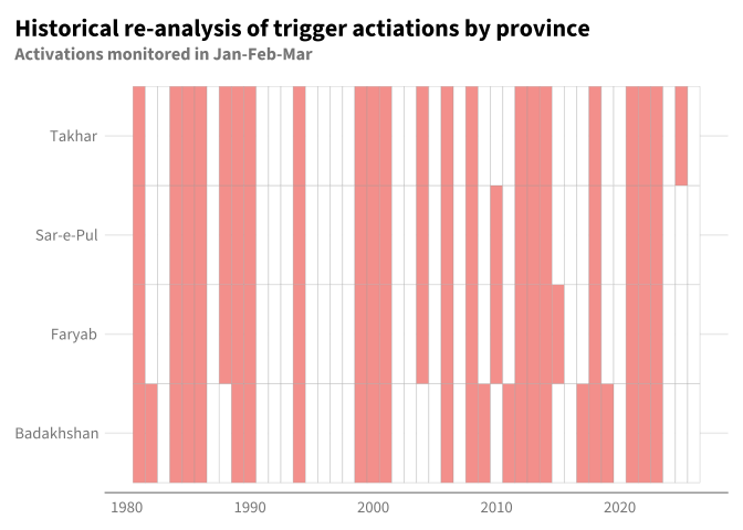
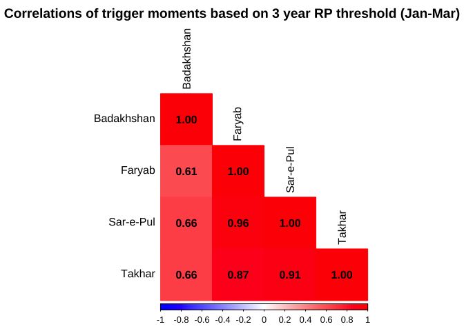
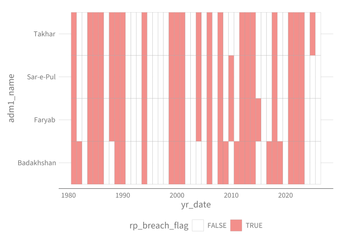
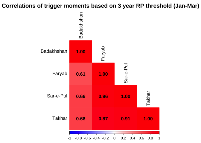
Look at historical re-analysis of trigger activation by region/AOI to understand co-occurrence/correlation structures. The takeaway here is that the province level pre-season SEAS triggers are highly correlated with Badakhshan as a bit of an outlier. It was hypothesized that this could be due to the Eastern district (Wakhan). However, removing it did little to change the overall historical re-analysis results.

df_seas5_aoi4_yearly_classified <- df_sea5_mam_aoi4_classified |>
    filter(month(issued_date) %in% c(1, 2, 3)) |>
    group_by(
        yr_date = floor_date(issued_date, "year"),
        # parameter,
        iso3,
        adm1_name,
        pcode,
    ) |>
    summarise(
        rp_breach_flag = any(flag),
        rp_breach_class = case_when(
            any(flag & rp == 5) ~ "5 year RP",
            any(flag & rp == 4) ~ "4 year RP",
            any(flag & rp == 3) ~ "3 year RP",
            .default = "1-3 year RP"
        )
    )

df_seas5_aoi4_yearly_classified |>
    ggplot(
        aes(x = yr_date, y = adm1_name, fill = rp_breach_flag)
    ) +
    geom_tile(color = "darkgrey") +
    scale_fill_manual(
        values = c("TRUE" = hdx_hex("tomato-light"), "FALSE" = "white")
    )

A degree of correlation is apparent - let’s dig in a little.

Here are the correlatoin coefficients of trigger years

ldf_yearly_classified <-
    list(
        "AOI4" = df_sea5_mam_aoi4_classified,
        "AOI4_NO_WAKHAN" = df_seas5_mam_aoi4_no_wakhan_classified
    ) |>
    map(
        \(dft){
            dft |>
                filter(month(issued_date) %in% c(1, 2, 3)) |>
                group_by(
                    yr_date = floor_date(issued_date, "year"),
                    # parameter,
                    iso3,
                    adm1_name,
                    pcode,
                ) |>
                summarise(
                    rp_breach_flag = any(flag),
                    rp_breach_class = case_when(
                        any(flag & rp == 5) ~ "5 year RP",
                        any(flag & rp == 4) ~ "4 year RP",
                        any(flag & rp == 3) ~ "3 year RP",
                        .default = "1-3 year RP"
                    )
                )
        }
    )

lcorr <- ldf_yearly_classified |>
    map(
        \(dft){
            dft_wide <- dft |>
                filter(
                    adm1_name != "Badghis"
                ) |>
                pivot_wider(
                    id_cols = yr_date,
                    names_from = "adm1_name",
                    values_from = "rp_breach_flag"
                )

            cor(dft_wide[, -1])
        }
    )

lp_tile <- imap(ldf_yearly_classified, \(dft, nmt){
    pt <- dft |>
        filter(adm1_name != "Badghis") |>
        ggplot(
            aes(x = yr_date, y = adm1_name, fill = rp_breach_flag)
        ) +
        geom_tile(color = "darkgrey") +
        scale_fill_manual(
            values = c("TRUE" = hdx_hex("tomato-light"), "FALSE" = "white")
        ) +
        labs(
            title = "Historical re-analysis of trigger actiations by province",
            subtitle = "Activations monitored in Jan-Feb-Mar"
        ) +
        theme(
            axis.title = element_blank(),
            legend.title = element_blank(),
            legend.position = "none"
        )
    if (nmt == "AOI4_NO_WAKHAN") {
        capt_text <- "Wakhan removed from Badakhshan"
        pt <- pt +
            labs(
                caption = capt_text
            )
    }
    return(pt)
})



corrplot::corrplot(lcorr$AOI4,
    method = "color", # Use colored tiles
    type = "lower", # Show only the lower triangle
    col = colorRampPalette(c("blue", "white", "red"))(200), # Color gradient
    addCoef.col = "black", # Add correlation coefficients
    title = "Correlations of trigger moments based on 3 year RP threshold (Jan-Mar)",
    tl.col = "black", # Variable labels color
    mar = c(0, 0, 2, 0)
) # A

We can see the years stacked up historically as well:

lp_tile$AOI4

We see that Badakhshan seems to be a bit of an outlier. It was therefore hypothesized that this could be due to the unique geography/env of th eastern district Wakhan.

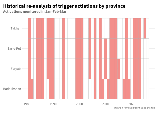
Therefore let’s see what would happen if we removed Wakhan from Badakhshan.

Results show no difference when we remove Wakhan. While thresholds and aggregated amounts change, the years of activation don’t. While this may not be true at all trigger moments, but rather just in the J-F-M aggregate form. It does not seem like a particularly useful avenue to pursue

corrplot::corrplot(
    lcorr$AOI4_NO_WAKHAN,
    method = "color", # Use colored tiles
    type = "lower", # Show only the lower triangle
    col = colorRampPalette(c("blue", "white", "red"))(200), # Color gradient
    addCoef.col = "black", # Add correlation coefficients
    title = "Correlations of trigger moments based on 3 year RP threshold (Jan-Mar)",
    tl.col = "black", # Variable labels color
    mar = c(0, 0, 2, 0)
) #

lp_tile$AOI4_NO_WAKHAN

# some somewhat useful exploratory plots used in a more exploratory phase
# i believe the've lost relevancy by now so setting `eval: false`

num_trig_palette <- c(
    "0" = "#ffffff",
    "1" = "#ffcccc",
    "2" = "#ff6666",
    "3" = "#ff3333",
    "4" = "#cc0000"
)
box::use(ggiraph[...], glue[...])
lp_tile2 <- ldf_yearly_classified |>
    map(
        \(dft){
            dft |>
                filter(
                    adm1_name != "Badghis"
                ) |>
                group_by(
                    yr_date
                ) |>
                mutate(
                    `# concurrent triggers` = factor(ifelse(rp_breach_flag, sum(rp_breach_flag), 0), levels = c("0", "1", "2", "3", "4"))
                ) |>
                ungroup() |>
                ggplot(
                    aes(x = yr_date, y = adm1_name, fill = `# concurrent triggers`),
                    color = "darkgrey"
                ) +
                geom_tile_interactive(color = "black", aes(tooltip = glue("{year(yr_date)}"))) +
                scale_fill_manual(
                    values = num_trig_palette
                ) +
                theme(
                    axis.title = element_blank()
                )
        }
    )

girafe(ggobj = lp_tile2$AOI4)
girafe(ggobj = lp_tile2$AOI4_NO_WAKHAN)

Results above are sufficient to inform our decisions on types of allocation models that could make sense which we will explore in the subsequent sectinos

10.3 Option 1A - 4 AOIs

All 4 provinces are monitored independently. Allocations split by province so each allocatio is only associated w/ the RPs for the respective province

# Some very specific function to output empirical joint activation rate/
# joint RPs in a standardized format. Not generic functions, but useful for
# reducing code downstream

joint_rps <- function(df, by) {
    df |>
        group_by(
            # combo of across() and any_of()  inside `group_by()
            # allows dynamic grouping based on whatever variables are present
            across(
                any_of(by)
            ),
            yr_date = floor_date(issued_date, "year")
        ) |>
        summarise(
            any_jan = any(flag & pub_mo == "Jan"),
            any_feb = any(flag & pub_mo == "Feb"),
            any_mar = any(flag & pub_mo == "Mar"),
            any_jan_feb = any(flag & pub_mo %in% c("Jan", "Feb")),
            any_feb_mar = any(flag & pub_mo %in% c("Feb", "Mar")),
            any_jan_feb_mar = any(flag & pub_mo %in% c("Jan", "Feb", "Mar")),
            .groups = "drop_last"
        ) |>
        # group_by(
        #   across(any_of(by))
        # ) |>
        summarise(
            across(
                starts_with("any_"), \(x) 1 / mean(x)
            ),
            .groups = "drop"
        )
}


# gt - {gt} - table package
gt_jrp <- function(
    df,
    strata = c("adm1_name" = "Province"),
    gt_pal) {
    gt_base <- df |>
        mutate(
            type = glue("{rp} year RP")
        ) |>
        group_by(type) |>
        gt() |>
        cols_hide(
            columns = any_of(c("iso3", "pcode", "rp"))
        )
    if (!is.null(strata)) {
        gt_base <- gt_base |>
            cols_label(
                !!sym(names(strata)) := strata
            )
    }
    gt_labelled <- gt_base |>
        cols_label(
            any_jan = "Jan",
            any_feb = "Feb",
            any_mar = "Mar",
            any_jan_feb = "Jan + Feb",
            any_feb_mar = "Feb + Mar",
            any_jan_feb_mar = "Jan + Feb + Mar"
        ) |>
        tab_spanner(
            columns = c("any_jan", "any_feb", "any_mar"),
            label = "1 activation moment"
        ) |>
        tab_spanner(columns = c("any_jan_feb", "any_feb_mar"), label = "2 activation moments") |>
        tab_spanner(columns = c("any_jan_feb_mar"), label = "3 activation moments") |>
        fmt_number(decimals = 1)

    gt_labelled |>
        data_color(
            columns = names(strata),
            colors = gt_pal,
            target_columns = everything()
        )
}

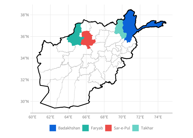
gdf_adm1_aoi <- lgdf$afg_adm1 |>
    filter(
        ADM1_EN %in% aoi_adm1
    )
ggplot() +
    geom_sf(data = lgdf$afg_adm1, color = "lightgrey", fill = NA) +
    geom_sf(data = gdf_adm1_aoi, aes(color = ADM1_EN, fill = ADM1_EN)) +
    geom_sf(data = lgdf$afg_adm0, color = "black", fill = NA, linewidth = 1) +
    theme(
        legend.title = element_blank()
    )

# Calculate all Joint Return Period Sets

# 4 AOIs monitored independently - implies province level activation and
# allocation
df_jrp_aoi4 <- joint_rps(
    df_sea5_mam_aoi4_classified,
    by = c("rp", "iso3", "pcode", "adm1_name")
)

# 4 AOI monitored independently - 1 activation implies entire pre-season
# allocation
c("rp", "iso3", "pcode", "adm1_name", "region")

[1] "rp"        "iso3"      "pcode"     "adm1_name" "region"   

gt_jrp(df_jrp_aoi4,
    strata = c("adm1_name" = "Province"),
    gt_pal = c("#66B0EC", "#78D9D1", "#FCE0DE", "#D2F2F0")
) |>
    tab_header(
        title = "SEAS5 - Joint Return Periods",
        subtitle = "Scenario: 1 Province level activations and allocations"
    )

SEAS5 - Joint Return Periods
Scenario: 1 Province level activations and allocations
Province	1 activation moment			2 activation moments		3 activation moments
	Jan	Feb	Mar	Jan + Feb	Feb + Mar	Jan + Feb + Mar
3 year RP
Badakhshan	3.1	3.3	3.3	2.3	2.2	1.9
Takhar	3.3	3.1	3.3	2.6	2.2	2.1
Sar-e-Pul	3.3	3.3	3.3	2.7	2.3	2.1
Faryab	3.3	3.3	3.3	2.7	2.3	2.0
4 year RP
Badakhshan	4.2	4.2	4.2	2.9	2.7	2.2
Takhar	4.2	4.2	4.2	3.1	2.7	2.3
Sar-e-Pul	4.2	4.2	4.2	3.1	2.7	2.3
Faryab	4.2	4.2	4.2	2.9	2.7	2.2
5 year RP
Badakhshan	5.8	5.8	5.8	3.5	3.5	2.7
Takhar	5.8	5.8	5.8	3.8	3.5	2.7
Sar-e-Pul	5.8	5.8	5.8	3.5	3.3	2.4
Faryab	5.8	5.8	5.8	3.8	3.3	2.6

10.4 Option 1B - 4 AOIs - All In

All 4 provinces monitored independently, but if 1 trigger threshold is met, the entire pre-season allocation would be made

df_jrp_aoi4_all_in <- joint_rps(
    df_sea5_mam_aoi4_classified,
    by = c("rp", "iso3")
)

gt_jrp(
    df_jrp_aoi4_all_in,
    strata = c("rp" = "RP"), gt_pal = c("#66B0EC", "#78D9D1", "#FCE0DE")
) |>
    tab_header(
        title = "SEAS5 - Joint Return Periods",
        subtitle = "Scenario 1b: Province level monitoring, but entire allocation upon 1 activation"
    )

SEAS5 - Joint Return Periods
Scenario 1b: Province level monitoring, but entire allocation upon 1 activation
1 activation moment			2 activation moments		3 activation moments
Jan	Feb	Mar	Jan + Feb	Feb + Mar	Jan + Feb + Mar
3 year RP
2.2	2.3	2.2	1.9	1.7	1.6
4 year RP
2.9	2.9	2.6	2.3	1.8	1.7
5 year RP
3.3	4.2	3.3	2.7	2.3	1.9

10.5 Option 2: 4 AOIs - grouped allocations

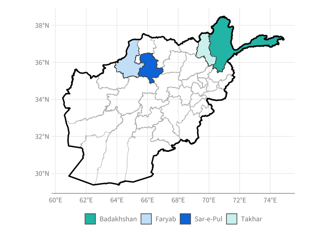
Each province monitored independently, but allocation split into 2 groups: North Central and North East. If a province in either group triggers the full allocation for that group is distributed.

pal_scenario_2 <- c(
    "Faryab" = hdx_hex("sapphire-ultra-light"),
    "Sar-e-Pul" = hdx_hex("sapphire-hdx"),
    "Takhar" = hdx_hex("mint-ultra-light"),
    "Badakhshan" = hdx_hex("mint-hdx")
)

ggplot() +
    geom_sf(data = lgdf$afg_adm1, color = "grey", fill = NA) +
    geom_sf(
        data = gdf_adm1_aoi,
        aes(fill = ADM1_EN)
    ) +
    scale_fill_manual(
        values = pal_scenario_2
    ) +
    geom_sf(data = lgdf$afg_adm0, color = "black", fill = NA, linewidth = 1) +
    theme(
        legend.title = element_blank()
    )

# 2 AOIs monitored independently (province merged in North Central & North East)
# these AOIs are made by aggregating provinces into 2 groups


df_jrp_aoi4_2_allocations <- joint_rps(
    df_sea5_mam_aoi4_classified |>
        mutate(
            region = ifelse(
                adm1_name %in% c("Faryab", "Sar-e-Pul"), "North Central", "North East"
            )
        ),
    by = c("iso3", "rp", "region")
)

gt_jrp(
    df_jrp_aoi4_2_allocations,
    strata = c("region" = "Region"),
    gt_pal = c(pal_scenario_2[1], pal_scenario_2[3])
)

Region	1 activation moment			2 activation moments		3 activation moments
	Jan	Feb	Mar	Jan + Feb	Feb + Mar	Jan + Feb + Mar
3 year RP
North Central	3.1	3.1	3.3	2.6	2.2	2.0
North East	2.6	2.6	2.4	2.1	1.8	1.7
4 year RP
North Central	3.5	3.3	3.5	2.7	2.3	2.1
North East	3.5	3.5	3.1	2.6	2.2	1.9
5 year RP
North Central	5.1	4.6	5.1	3.3	2.9	2.4
North East	4.6	4.6	4.2	3.1	2.9	2.3

10.6 Option 3 - 2 AOIs

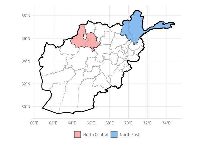
The 4 AOIs are grouped into 2 AOIs which are monitored independently at the group level rather than province level. If the thresholds for the new AOI/group is breached the allocation for that group is distributed.

pal_scenario_3 <- c(
    "North Central" = hdx_hex("tomato-light"),
    "North East" = hdx_hex("sapphire-light")
)
gdf_region_aoi <- gdf_adm1_aoi |>
    mutate(
        region = ifelse(ADM1_EN %in% c("Faryab", "Sar-e-Pul"), "North Central", "North East")
    ) |>
    group_by(region) |>
    summarise()

ggplot() +
    geom_sf(
        data = lgdf$afg_adm1, color = "grey", fill = NA
    ) +
    geom_sf(
        data = gdf_region_aoi,
        aes(fill = region), alpha = 0.7
    ) +
    scale_fill_manual(
        values = pal_scenario_3
    ) +
    geom_sf(data = lgdf$afg_adm0, color = "black", fill = NA, linewidth = 1) +
    theme(
        legend.title = element_blank()
    )

df_jrp_aoi2 <- joint_rps(
    df_seas5_region_aoi2_classified,
    by = c("rp", "iso3", "region")
)


gt_jrp(
    df_jrp_aoi2,
    strata = c("region" = "Region"),
    gt_pal = scales::alpha(pal_scenario_3, alpha = 0.5)
) |>
    tab_header(
        title = "SEAS5 - Joint Return Periods",
        subtitle = "Scenario: 4 Provinces grouped into 2 AOIs and monitored as 2 potential allocations "
    )

SEAS5 - Joint Return Periods
Scenario: 4 Provinces grouped into 2 AOIs and monitored as 2 potential allocations
Region	1 activation moment			2 activation moments		3 activation moments
	Jan	Feb	Mar	Jan + Feb	Feb + Mar	Jan + Feb + Mar
3 year RP
North Central	3.3	3.3	3.3	2.7	2.3	2.0
North East	3.3	3.1	3.1	2.4	2.1	2.0
4 year RP
North Central	4.2	4.2	4.2	2.9	2.9	2.3
North East	4.2	4.2	4.2	2.9	2.6	2.2
5 year RP
North Central	5.8	5.8	5.8	3.5	3.3	2.4
North East	5.1	5.8	5.8	3.5	3.3	2.4

10.7 Option 4A - 1 AOI

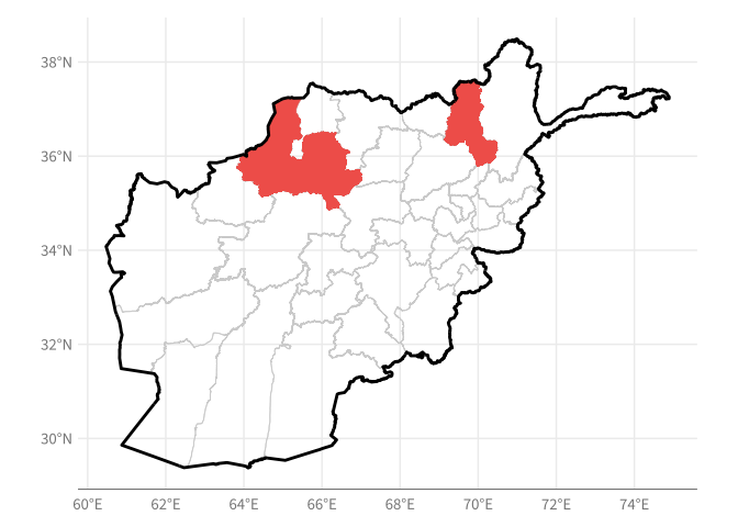
3 provinces (Takhar, Faryab, Sar-e-Pul) monitored as one AOI (polygons merged)

gdf_aoi_1 <- gdf_adm1_aoi |>
    filter(
        ADM1_EN %in% c("Faryab", "Sar-e-Pul", "Takhar")
    ) |>
    summarise()
ggplot() +
    geom_sf(
        data = lgdf$afg_adm1,
        color = "lightgrey",
        fill = NA,
        linewidth = 0.3
    ) +
    geom_sf(
        data = gdf_aoi_1,
        fill = hdx_hex("tomato-hdx"),
        alpha = 1,
        color = hdx_hex("tomato-hdx")
    ) +
    geom_sf(data = lgdf$afg_adm0, color = "black", fill = NA, linewidth = 1) +
    theme(
        legend.title = element_blank()
    )

# 1 AOI (3 provinces merged)

df_jrp_aoi1 <- joint_rps(df_seas5_mam_aoi1_classified, by = c("rp", "iso3"))

gt_jrp(
    df_jrp_aoi1,
    strata = c("rp" = "RP"),
    gt_pal = hdx_hex("tomato-ultra-light")
) |>
    tab_header(
        title = "SEAS5 - Joint Return Periods",
        subtitle = "Scenario: 3 Provinces monitored together as 1 AOI"
    )

SEAS5 - Joint Return Periods
Scenario: 3 Provinces monitored together as 1 AOI
1 activation moment			2 activation moments		3 activation moments
Jan	Feb	Mar	Jan + Feb	Feb + Mar	Jan + Feb + Mar
3 year RP
3.3	3.1	3.1	2.7	2.1	2.0
4 year RP
4.2	4.2	4.2	2.9	2.7	2.2
5 year RP
5.1	5.1	5.8	3.3	3.5	2.6

10.8 Option 4B - 3 AOIs - All in

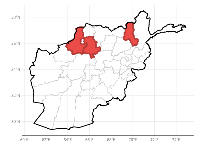
3 Provinces monitored independently, but if 1 threshold is breached it triggers entire pre-season allocation

# 3 AOIs monitored independently - 1 acitvation implies entire pre-season

gdf_adm1_aoi3 <- gdf_adm1_aoi |>
    filter(
        ADM1_EN %in% c("Faryab", "Sar-e-Pul", "Takhar")
    )

ggplot() +
    geom_sf(
        data = lgdf$afg_adm1,
        color = "lightgrey",
        fill = NA,
        linewidth = 0.5
    ) +
    geom_sf(
        data = gdf_adm1_aoi3,
        fill = hdx_hex("tomato-hdx"),
        alpha = 1,
        color = hdx_hex("tomato-dark"), linewidth = 1.5
    ) +
    geom_sf(data = lgdf$afg_adm0, color = "black", fill = NA, linewidth = 1) +
    theme(
        legend.title = element_blank()
    )

df_jrp_aoi3_all_in <- joint_rps(
    df_sea5_mam_aoi4_classified |>
        filter(
            adm1_name != "Badakhshan"
        ),
    by = c("rp", "iso3")
)

gt_jrp(
    df_jrp_aoi3_all_in,
    strata = c("rp" = "RP"),
    gt_pal = c(
        hdx_hex("tomato-ultra-light")
    )
) |>
    tab_header(
        title = "SEAS5 - Joint Return Periods",
        subtitle = "Scenario: 3 Provinces monitored independently, but 1 triggers all-in allocation"
    )

SEAS5 - Joint Return Periods
Scenario: 3 Provinces monitored independently, but 1 triggers all-in allocation
1 activation moment			2 activation moments		3 activation moments
Jan	Feb	Mar	Jan + Feb	Feb + Mar	Jan + Feb + Mar
3 year RP
2.6	2.7	2.9	2.3	2.1	1.9
4 year RP
3.1	3.3	3.3	2.7	2.2	2.0
5 year RP
3.8	4.6	4.2	3.1	2.7	2.2

10.9 RP Disussion

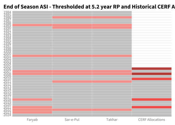
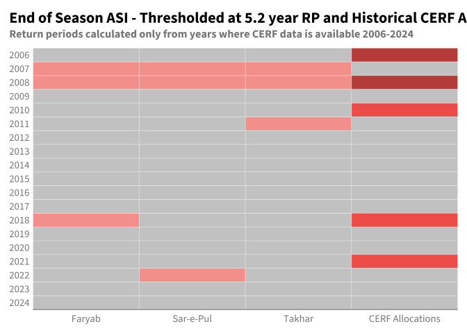
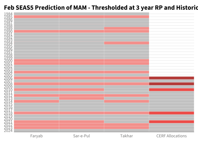
Why are we choosing a 3 year RP? Well we do see that CERF allocatoins since 2008 have a rougly 1 in 3 year RP and they line up decently with

aoi_adm1 <- c(
    "Takhar",
    # "Badakhshan",
    # "Badghis",
    "Sar-e-Pul",
    "Faryab"
)
df_fao <- loaders$load_fao_vegetation_data()
df_cerf <- cumulus::blob_read("ds-aa-afg-drought/raw/vector/afg_drought_cerf_allocations.xlsx") |>
    clean_names() |>
    mutate(
        allocation_date = as_date(allocation_date)
    )

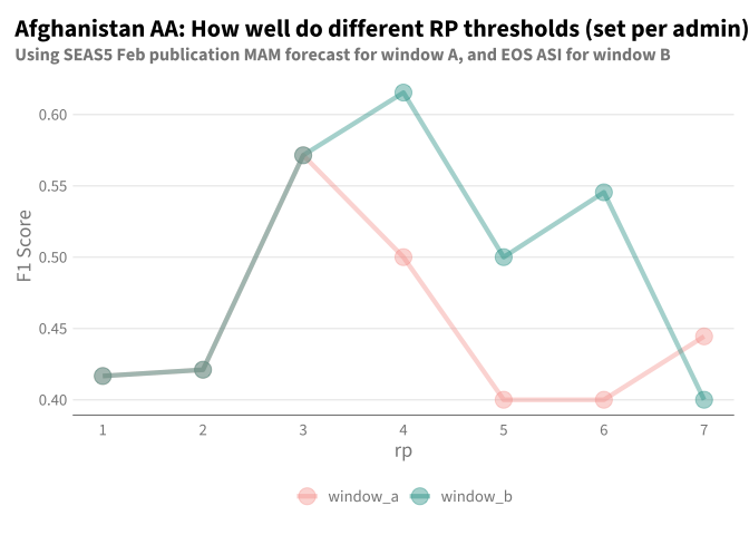
# if you do play around w/ this number it does look like it peaks out around 4... which equate to a joint RP of around 3
# w/ rp at 5 u miss 2006 activatoin
rp_compare <- 5.2

df_asi_eos_full <- df_fao |>
    clean_names() |>
    mutate(
        date = as_date(date),
        yr_season = floor_date(date, "year")
    ) |>
    filter(
        adm1_name %in% aoi_adm1,
        year(date) <= 2024,
        month(date) == 5,
        dekad == 3,
        parameter == "asi"
    ) |>
    utils$threshold_var(
        var = "value",
        by = c("adm1_name"),
        rp_threshold = rp_compare
    ) |>
    mutate(
        yr = year(yr_season)
    ) |>
    rename(
        strata = adm1_name
    )
df_asi_eos_shortened <- df_fao |>
    clean_names() |>
    mutate(
        date = as_date(date),
        yr_season = floor_date(date, "year")
    ) |>
    filter(
        adm1_name %in% aoi_adm1,
        year(date) <= 2024,
        year(date) >= 2006,
        month(date) == 5,
        dekad == 3,
        parameter == "asi"
    ) |>
    utils$threshold_var(
        var = "value",
        by = c("adm1_name"),
        rp_threshold = rp_compare
    ) |>
    mutate(
        yr = year(yr_season)
    ) |>
    rename(
        strata = adm1_name
    )


df_cerf_yr <- df_cerf |>
    group_by(yr = year(allocation_date)) |>
    summarise(
        n = n()
    ) |>
    complete(
        yr = 2006:2024,
        fill = list(n = 0)
    )

historical view of end of season ASI vs CERF allocation

# ASI vs
bind_rows(
    df_asi_eos_full,
    df_cerf_yr |>
        mutate(
            strata = "CERF Allocations",
            value_flag = n > 0
        )
) |>
    mutate(
        value_fill = case_when(
            value_flag == F ~ "no activations",
            value_flag == T & strata != "CERF Allocations" ~ "activation",
            value_flag == T & strata == "CERF Allocations" & n == 1 ~ "1 activation",
            value_flag == T & strata == "CERF Allocations" & n == 2 ~ "2 activations",
            .default = "?"
        ),
        strata = factor(strata, c("Faryab", "Sar-e-Pul", "Takhar", "CERF Allocations")),
    ) |>
    ggplot(
        aes(x = strata, y = yr, fill = value_fill)
    ) +
    geom_tile(color = "white") +
    scale_fill_manual(
        values = c(
            "no activations" = hdx_hex("grey-medium"),
            "activation" = hdx_hex("tomato-light"),
            "1 activation" = hdx_hex("tomato-hdx"),
            "2 activations" = hdx_hex("tomato-dark")
        )
    ) +
    scale_y_reverse(expand = c(0, 0), breaks = 1984:2024) +
    scale_x_discrete(expand = c(0, 0)) +
    theme(
        axis.title = element_blank(),
        legend.position = "none"
    ) +
    labs(
        title = glue("End of Season ASI - Thresholded at {rp_compare} year RP and Historical CERF Activations")
    )

bind_rows(
    df_asi_eos_shortened,
    df_cerf_yr |>
        mutate(
            strata = "CERF Allocations",
            value_flag = n > 0
        )
) |>
    mutate(
        value_fill = case_when(
            value_flag == F ~ "no activations",
            value_flag == T & strata != "CERF Allocations" ~ "activation",
            value_flag == T & strata == "CERF Allocations" & n == 1 ~ "1 activation",
            value_flag == T & strata == "CERF Allocations" & n == 2 ~ "2 activations",
            .default = "?"
        ),
        strata = factor(strata, c("Faryab", "Sar-e-Pul", "Takhar", "CERF Allocations")),
    ) |>
    ggplot(
        aes(x = strata, y = yr, fill = value_fill)
    ) +
    geom_tile(color = "white") +
    scale_fill_manual(
        values = c(
            "no activations" = hdx_hex("grey-medium"),
            "activation" = hdx_hex("tomato-light"),
            "1 activation" = hdx_hex("tomato-hdx"),
            "2 activations" = hdx_hex("tomato-dark")
        )
    ) +
    scale_y_reverse(expand = c(0, 0), breaks = 1984:2024) +
    scale_x_discrete(expand = c(0, 0)) +
    theme(
        axis.title = element_blank(),
        legend.position = "none"
    ) +
    labs(
        title = glue("End of Season ASI - Thresholded at {rp_compare} year RP and Historical CERF Activations"),
        subtitle = "Return periods calculated only from years where CERF data is available 2006-2024"
    )

historical view of Feb SEAS5 prediction for MAM vs CERF allocation

rp_compare <- 3

df_asi_validation <- df_fao |>
    clean_names() |>
    mutate(
        date = as_date(date),
        yr_season = floor_date(date, "year")
    ) |>
    filter(
        adm1_name %in% aoi_adm1,
        year(date) <= 2024,
        month(date) == 5,
        dekad == 3,
        parameter == "asi"
    )

df_compiled_indicators <- loaders$load_compiled_indicators(aoi_adm1 = aoi_adm1)

df_seas5_mam <- df_compiled_indicators |>
    filter(
        parameter == "SEAS5-MAM"
    )


df_seas5_mam |>
    mutate(
        yr = year(yr_season),
        value_flag = rp_relevant_direction >= rp_compare
    ) |>
    rename(
        strata = adm1_name
    ) |>
    bind_rows(
        df_cerf_yr |>
            mutate(
                strata = "CERF Allocations",
                value_flag = n > 0
            )
    ) |>
    mutate(
        value_fill = case_when(
            value_flag == F ~ "no activations",
            value_flag == T & strata != "CERF Allocations" ~ "activation",
            value_flag == T & strata == "CERF Allocations" & n == 1 ~ "1 activation",
            value_flag == T & strata == "CERF Allocations" & n == 2 ~ "2 activations",
            .default = "?"
        ),
        strata = factor(strata, c("Faryab", "Sar-e-Pul", "Takhar", "CERF Allocations")),
    ) |>
    ggplot(
        aes(x = strata, y = yr, fill = value_fill)
    ) +
    geom_tile(color = "white") +
    scale_fill_manual(
        values = c(
            "no activations" = hdx_hex("grey-medium"),
            "activation" = hdx_hex("tomato-light"),
            "1 activation" = hdx_hex("tomato-hdx"),
            "2 activations" = hdx_hex("tomato-dark")
        )
    ) +
    scale_y_reverse(expand = c(0, 0), breaks = 1984:2024) +
    scale_x_discrete(expand = c(0, 0)) +
    theme(
        axis.title = element_blank(),
        legend.position = "none"
    ) +
    labs(
        title = glue("Feb SEAS5 Prediction of MAM - Thresholded at {rp_compare} year RP and Historical CERF Activations")
    )

quantitative analysis: optimal RP thresholds for prediction of CERF allocation

df_windows_flagged_adm1 <- map(1:7, \(rp_temp){
    # rp_temp <- 2
    df_window_b_flag <- df_asi_validation |>
        utils$threshold_var(
            var = "value",
            by = c("adm1_name"),
            rp_threshold = rp_temp
        ) |>
        mutate(
            yr = year(yr_season),
            rp = rp_temp
        ) |>
        rename(
            window_b_flag = value_flag
        ) |>
        select(yr, rp, adm1_name, window_b_flag)

    df_seas5_mam |>
        mutate(
            yr = year(yr_season)
        ) |>
        arrange(yr)

    df_window_a_flag <- df_seas5_mam |>
        filter(pub_mo_label == "Feb") |>
        mutate(
            yr = year(yr_season),
            window_a_flag = rp_relevant_direction >= rp_temp,
            rp = rp_temp
        ) |>
        select(yr, rp, adm1_name, window_a_flag)

    left_join(df_window_b_flag, df_window_a_flag, by = c("yr", "adm1_name", "rp"))
}) |>
    list_rbind()

df_asi_cerf_joined <- df_windows_flagged_adm1 |>
    group_by(
        yr, rp
    ) |>
    # count(value_flag)
    summarise(
        window_a_flag = any(window_a_flag),
        window_b_flag = any(window_b_flag)
    ) |>
    inner_join(
        df_cerf_yr |>
            mutate(
                cerf_flag = n > 0
            )
    )


df_optimal_window_a <- df_asi_cerf_joined |>
    group_by(
        rp
    ) |>
    mutate(
        across(ends_with("flag"), \(x) fct_relevel(as_factor(x), "TRUE", "FALSE"))
    ) |>
    yardstick::f_meas(truth = window_a_flag, estimate = cerf_flag) |>
    mutate(
        window = "window_a"
    )

df_optimal_window_b <- df_asi_cerf_joined |>
    group_by(
        rp
    ) |>
    mutate(
        across(ends_with("flag"), \(x) fct_relevel(as_factor(x), "TRUE", "FALSE"))
    ) |>
    yardstick::f_meas(truth = window_b_flag, estimate = cerf_flag) |>
    mutate(
        window = "window_b"
    )

bind_rows(
    df_optimal_window_a,
    df_optimal_window_b
) |>
    ggplot(
        aes(x = rp, y = .estimate, group = window, color = window)
    ) +
    geom_line(linewidth = 1.5, alpha = 0.4) +
    geom_point(alpha = 0.4, size = 5) +
    scale_x_continuous(breaks = 1:7) +
    labs(
        title = "Afghanistan AA: How well do different RP thresholds (set per admin) predict CERF allocation",
        subtitle = "Using SEAS5 Feb publication MAM forecast for window A, and EOS ASI for window B",
        y = "F1 Score"
    ) +
    scale_color_manual(
        values = c("window_a" = hdx_hex("tomato-light"), "window_b" = hdx_hex("mint-dark"))
    ) +
    theme(
        legend.title = element_blank()
    )

10.10 Remaining Steps

• CERF/OCHA AFG coordinate partners to decide on pre-season trigger moments and allocation model
• CERF/OCHA AFG decide if March fits into pre-season or mid/post-season allocation bucket