3 AOI Selection - Prioritization

3.1 Intro

Preliminary work

This document contains exploratory work done to support area targeting for drought monitoring and AA activity implementation. Initially the discussion centered around drought monitoring over the winter wheat agricultural season in Afghanistan, later this was revised to the Spring wheat growing season

While targeting decisions should ultimately be made by in-country experts and implementing partners to reflect operational realities, this document aims to explore several additional data sets to support this process and encourage discussion.

The document focuses on 3 main data sets:

Winter wheat/Spring wheat crops mask (TBD)
Rainfall (CHIRPS)
Food Insecurity (IPC Phase Classification)

3.1.1 Key Takeaways

To date no winter/spring wheat crop mask provided. Therefore, the identification of key wheat growing areas has been left to in-country experts
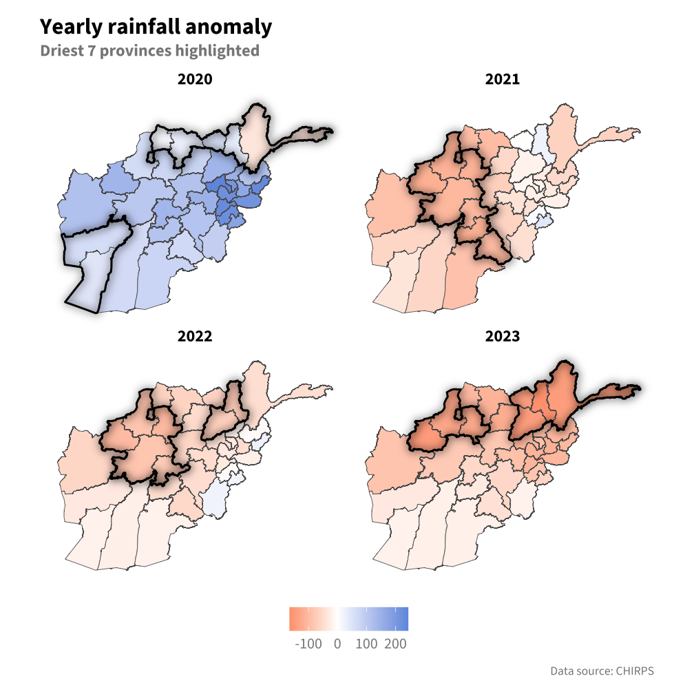
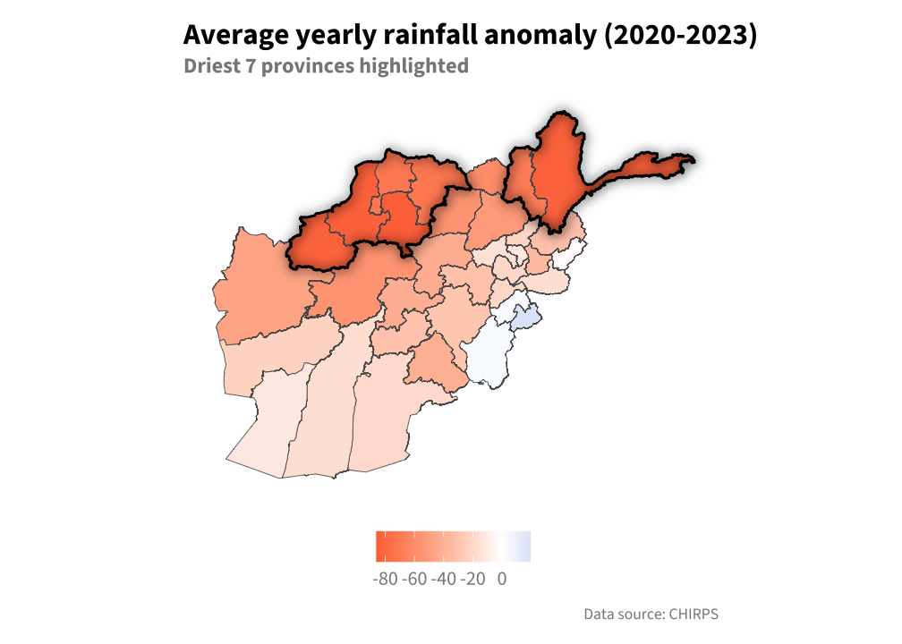
Rainfall analysis provides useful clustering of provinces based on historical scarcity in alignment with general feedback from in-country partners
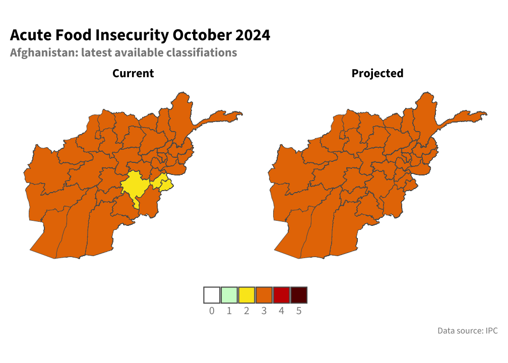
Up to date IPC Phase Classifications have not shown to be useful for prioritization due to homogeneity of the latest classification which offers little discriminatory power for this project

Working group feedback:

The initial group decision was to focus the pilot on Faryab province in the north
As of December 2024, the group has tentatively decided to expand to include Faryab ,Takhar, Badakhshan, Badghis, Sar-e-Pul provinces.

Code

box::use(
    dplyr[...],
    ggplot2[...],
    lubridate[...],
    purrr[...],
    tidyr[...],
    stringr[...],
    readr[...],
    gghdx[...],
    janitor[...],
    scales[...],
    sf[...],
    geoarrow[...],
    forcats[...],
    ggfx[...],
    patchwork[...]
)

box::use(ggiraph)
box::use(ripc)
box::use(cumulus)

box::use(blob = .. / R / blob_connect)

gghdx()

# load admin boundaries
gdf_adm1 <- cumulus::blob_read(
    name = "ds-aa-afg-drought/raw/vector/afg_admbnda_agcho_adm1.parquet",
    container = "projects", as_data_frame = FALSE
) |>
    st_as_sf() |>
    clean_names() |>
    select(matches("adm\\d_[pe]"))

gdf_adm2 <- cumulus::blob_read(
    name = "ds-aa-afg-drought/raw/vector/afg_admbnda_agcho_adm2.parquet",
    container = "projects", as_data_frame = FALSE
) |>
    st_as_sf() |>
    clean_names() |>
    select(matches("adm\\d_[pe]"))

# gdf_adm1 <- cumulus$download_fieldmaps_sf(iso3 = "AFG", layer = "afg_adm1")$afg_adm1 |>
#     clean_names() |>
#     select(matches("adm\\d_[pe]"))
#
#
# gdf_adm2 <- cumulus$download_fieldmaps_sf(iso3 = "AFG", layer = "afg_adm2")$afg_adm2 |>
#     clean_names() |>
#     select(matches("adm\\d_[pe]"))

# load chirps rainfall
fps <- blob$proj_blob_paths()

df_chirps_adm2 <- cumulus$blob_read(
    name = fps$DF_ADM2_CHIRPS_WFP,
    container = "projects",
    stage = "dev",
    progress_show = FALSE
)

3.2 Winter Wheat

Data source: TBD (waiting for officially recommended winter wheat crop mask layer).

Idea: On basis that activities/framework will be centered around winter wheat agricultural season we should target areas where winter wheat is grown. If we have a crop mask we could analyze total area/% area growing winter wheat at an admin level and use that as an input for the targeting/prioritization analysis.

3.3 Rainfall

Data source: CHIRPS

Code

# Get area of adm2 as % of adm1 for weighting
df_adm2_w_area <- gdf_adm2 %>%
    mutate(
        area = st_area(.)
    ) |>
    group_by(adm1_pcode, adm1_en) %>%
    mutate(
        adm1_area = sum(area)
    ) |>
    ungroup() |>
    mutate(
        pct_area = area / adm1_area
    ) |>
    st_drop_geometry()

# get monthly rainfall by admin 2
df_chirps_monthly_adm2 <- df_chirps_adm2 |>
    mutate(
        mo_date = floor_date(date, "month"), .before = "date"
    ) |>
    group_by(
        across(
            matches("adm\\d_[pe]")
        ),
        mo_date
    ) |>
    summarise(
        precip = sum(rfh)
    ) |>
    left_join(
        df_adm2_w_area
    )


# aggregate to admin 1
df_chirps_monthly_adm1 <- df_chirps_monthly_adm2 |>
    group_by(
        across(
            matches("adm[01]_[pe]")
        ),
        mo_date
    ) |>
    summarise(
        precip = weighted.mean(x = as.numeric(precip), w = as.numeric(pct_area)),
        .groups = "drop"
    )


# aggregate to yearly
df_chirps_yearly_adm1 <- df_chirps_monthly_adm1 |>
    group_by(
        across(
            matches("adm\\d_[pe]")
        ),
        yr_date = floor_date(mo_date, "year")
    ) |>
    summarise(
        precip = sum(precip)
    )



baseline_years <- c(1981:2020)

# get average precip per year per admin using baseline
yearly_baseline_avg <- df_chirps_yearly_adm1 |>
    filter(
        year(yr_date) %in% baseline_years
    ) |>
    group_by(
        across(
            matches("adm\\d_[pe]")
        )
    ) |>
    summarise(
        avg_precip = mean(precip)
    )


# calculate anomaly
df_chirps_adm1_anomaly <- df_chirps_yearly_adm1 |>
    left_join(
        yearly_baseline_avg
    ) |>
    mutate(
        anom_abs = precip - avg_precip
    )



gdf_adm1_ranked <- gdf_adm1 |>
    left_join(
        df_chirps_adm1_anomaly |>
            filter(year(yr_date) %in% c(2020:2023)) |>
            group_by(
                yr_date
            ) |>
            arrange(
                yr_date,
                desc(-anom_abs)
            ) |>
            mutate(
                yr = as_factor(year(yr_date)),
                rank = row_number(),
                top5_dry = rank %in% c(1:7),
                top5_anom = if_else(top5_dry, anom_abs, NA_real_)
            )
    )


limit <- max(abs(gdf_adm1_ranked$top5_anom)) * c(-1, 1)

gdf_top5_diss <- gdf_adm1_ranked |>
    group_by(yr) |>
    filter(top5_dry) |>
    summarise()

Code

ggplot() +
    ggiraph$geom_sf_interactive(
        data = gdf_adm1_ranked,
        aes(
            fill = anom_abs,
            tooltip = adm1_en
        ),
        show.legend = c(color = FALSE, fill = TRUE)
    ) +
    with_shadow(
        geom_sf(
            data = gdf_top5_diss,
            # aes(fill= diff),
            fill = NA,
            alpha = 1,
            color = "black",
            lwd = 0.7
        ),
        sigma = 3,
        x_offset = 0.5,
        y_offset = 0.25
    ) +
    scale_fill_gradient2(low = "#FD7446", high = "#709AE1") +
    facet_wrap(~yr) +
    labs(
        title = "Yearly rainfall anomaly",
        subtitle = "Driest 7 provinces highlighted",
        caption = "Data source: CHIRPS"
    ) +
    theme(
        legend.title = element_blank(),
        axis.text = element_blank(),
        panel.grid = element_blank(),
        axis.line.x.bottom = element_blank()
    )

Code

gdf_adm1_ranked_overall <- gdf_adm1_ranked |>
    mutate(
        # these weights are subjective first go
        # rationale for weighting is that more recent years
        # should be weighted higher
        weights = case_when(
            yr == 2020 ~ 0.15,
            yr == 2021 ~ 0.2,
            yr == 2022 ~ 0.3,
            yr == 2023 ~ 0.35
        )
    ) |>
    group_by(
        across(matches("adm\\d_[pe]"))
    ) |>
    summarise(
        weighted_anom = weighted.mean(x = anom_abs, w = weights)
    ) |>
    ungroup() |>
    arrange(
        desc(-weighted_anom)
    ) |>
    mutate(
        rank = row_number(),
        top5_dry = rank %in% c(1:7),
        top5_anom = if_else(top5_dry, weighted_anom, NA_real_)
    )

gdf_top5_overall_diss <- gdf_adm1_ranked_overall |>
    filter(top5_dry) |>
    summarise()


ggplot() +
    geom_sf(
        data = gdf_adm1_ranked_overall,
        aes(fill = weighted_anom),
        show.legend = c(color = FALSE, fill = TRUE)
    ) +
    with_shadow(
        geom_sf(
            data = gdf_top5_overall_diss,
            # aes(fill= diff),
            fill = NA,
            alpha = 1,
            color = "black",
            lwd = 0.7
        ),
        sigma = 3,
        x_offset = 0.5,
        y_offset = 0.25
    ) +
    scale_fill_gradient2(low = "#FD7446", high = "#709AE1") +
    labs(
        title = "Average yearly rainfall anomaly (2020-2023)",
        subtitle = "Driest 7 provinces highlighted",
        caption = "Data source: CHIRPS"
    ) +
    theme(
        legend.title = element_blank(),
        axis.text = element_blank(),
        panel.grid = element_blank(),
        axis.line.x.bottom = element_blank()
    )

3.4 Food Insecurity (IPC)

Data source (IPC)

preliminary analysis - needs further validation

Code

# bugfix/pop-areas
ipc_get_areas_current_sf <- function(country) {
    # get full list of data sets
    ipc_pop_area <- ripc$ipc_get_population(country = country)$area

    # grab area analysis ids
    area_analysis_ids <- unique(ipc_pop_area$analysis_id)

    gdf_ipc_area <- map(
        area_analysis_ids,
        \(id_tmp){
            gdf_area <- ripc$ipc_get_areas(
                id = id_tmp,
                period = "C",
                return_format = "geojson"
            )

            gdf_area_merged <- gdf_area |>
                left_join(
                    ipc_pop_area |>
                        mutate(
                            analysis_id = as.character(analysis_id),
                            area_id = as.character(area_id)
                        ) |>
                        filter(
                            period == "current"
                        ) |>
                        select(
                            analysis_id,
                            area_id,
                            analysis_period_start,
                            analysis_period_end,
                            analysis_date,
                            title,
                            period
                        ),
                    by = c("analysis_id", "area_id"),
                    relationship = "one-to-one"
                )
            gdf_area_merged
        }
    )
    gdf_ipc_area |>
        list_rbind()
}

3.4.1 Latest IPC classification

Below we plot the latest IPC phase classifications produced:

Code

# having trouble with these API's during knitting. Therefore, I wrote output from this cell to to blob in next hidden chunk.

gdf_ipc_sf_current <- ipc_get_areas_current_sf(country = "AF")

latest_analysis_id <- gdf_ipc_sf_current |>
    filter(
        analysis_period_end == max(analysis_period_end)
    ) |>
    pull(
        analysis_id
    ) |>
    unique()


# hard codig this to id from Oct 2024 - was probably an earlier one when
# i first ran analysis - but this one still has same message
latest_analysis_id <- 72104327


# could put warning if latest_analysis_id > 1 -- here
gdf_ipc_sf_projected_latest <- ripc$ipc_get_areas(
    id = latest_analysis_id,
    period = "P",
    return_format = "geojson"
)


gdf_ipc_sf_current_latest <- gdf_ipc_sf_current |>
    filter(
        analysis_id == latest_analysis_id
    )


gdf_ipc_sf_latest <- bind_rows(
    gdf_ipc_sf_current_latest,
    gdf_ipc_sf_projected_latest
) |>
    mutate(
        ipc_period_label = if_else(ipc_period == "C", "Current", "Projected")
    )

Code

ipc_fill_pal <- c(
    "0" = "#FFFFFF",
    "1" = "#CDFACD",
    "2" = "#FAE61E",
    "3" = "#E67800",
    "4" = "#C80000",
    "5" = "#640000"
)

gdf_ipc_sf_latest_poly <- gdf_ipc_sf_latest |>
    filter(
        !(str_detect(st_geometry_type(geometry), "POINT"))
    ) |>
    st_as_sf() |>
    mutate(
        overall_phase = fct_relevel(
            fct_expand(
                as_factor(overall_phase),
                "0", "1", "2", "3", "4", "5"
            ),
            "0", "1", "2", "3", "4", "5"
        )
    )


p_title <- unique(gdf_ipc_sf_latest_poly$title)
p_title <- p_title[!is.na(p_title)]
ggplot() +
    geom_sf(
        data = gdf_ipc_sf_latest_poly,
        aes(
            fill = overall_phase,
        ), show.legend = c(fill = TRUE)
    ) +
    scale_fill_manual(
        values = ipc_fill_pal,
        drop = FALSE
    ) +
    facet_wrap(
        ~ipc_period_label
    ) +
    labs(
        title = p_title,
        subtitle = "Afghanistan: latest available classifiations",
        caption = "Data source: IPC"
    ) +
    guides(
        fill = guide_legend(
            label.position = "bottom",
            nrow = 1, byrow = TRUE
        )
    ) +
    theme(
        legend.title = element_blank(),
        axis.text = element_blank(),
        panel.grid = element_blank(),
        axis.line.x.bottom = element_blank(),
        legend.key.spacing = unit(0, "cm"),
        legend.text = element_text(margin = margin(t = 3))
    )

3.4.2 IPC Recent Years

Next we filter to last 5 years (2020-2024) to get an overview of how the situation has evolved recently

Code

gdf_ipc_sf_current_polys <- gdf_ipc_sf_current |>
    filter(
        !(str_detect(st_geometry_type(geometry), "POINT"))
    ) |>
    st_as_sf()


gdf_areas_filt <- gdf_ipc_sf_current_polys |>
    mutate(
        analysis_period_start_year = year(analysis_period_start),
        analysis_period_end_year = year(analysis_period_end),
        start_end = paste0(
            format(analysis_period_start, "%e %b %y"), "-",
            format(analysis_period_end, "%e %b %y")
        )
    ) |>
    filter(
        year(analysis_period_start) %in% 2020:2024
    )

df_lookup_factor_levels <- gdf_areas_filt |>
    st_drop_geometry() |>
    distinct(
        analysis_period_start,
        start_end
    ) |>
    arrange(
        analysis_period_start
    )


# factorize start_end so that factors are in same order as analysis_period_start
gdf_areas_filt <- gdf_areas_filt |>
    mutate(
        start_end = factor(start_end, levels = df_lookup_factor_levels$start_end),
        overall_phase_factor = fct_relevel(fct_expand(as_factor(overall_phase), "0", "1", "2", "3", "4", "5"), "0", "1", "2", "3", "4", "5")
    )

Code

# map each time period
ggplot() +
    geom_sf(
        data = gdf_areas_filt,
        aes(
            fill = overall_phase_factor,
        ), show.legend = c(fill = TRUE)
    ) +
    scale_fill_manual(
        values = ipc_fill_pal,
        drop = FALSE
    ) +
    facet_wrap(
        ~start_end
    ) +
    guides(
        fill = guide_legend(
            label.position = "bottom",
            nrow = 1, byrow = TRUE
        )
    ) +
    theme(
        legend.title = element_blank(),
        axis.text = element_blank(),
        panel.grid = element_blank(),
        axis.line.x.bottom = element_blank(),
        legend.key.spacing = unit(0, "cm"),
        legend.text = element_text(margin = margin(t = 3))
    )

3.4.3 Recent Years Aggregated

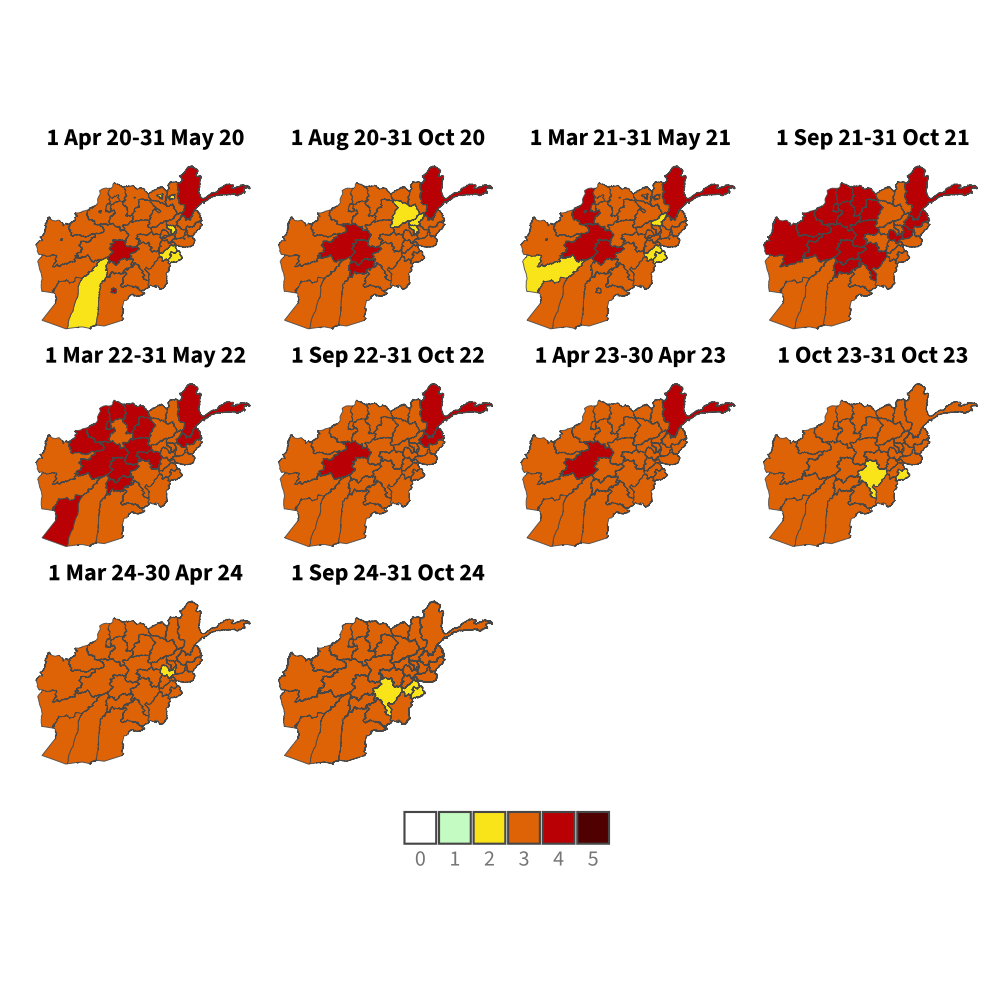
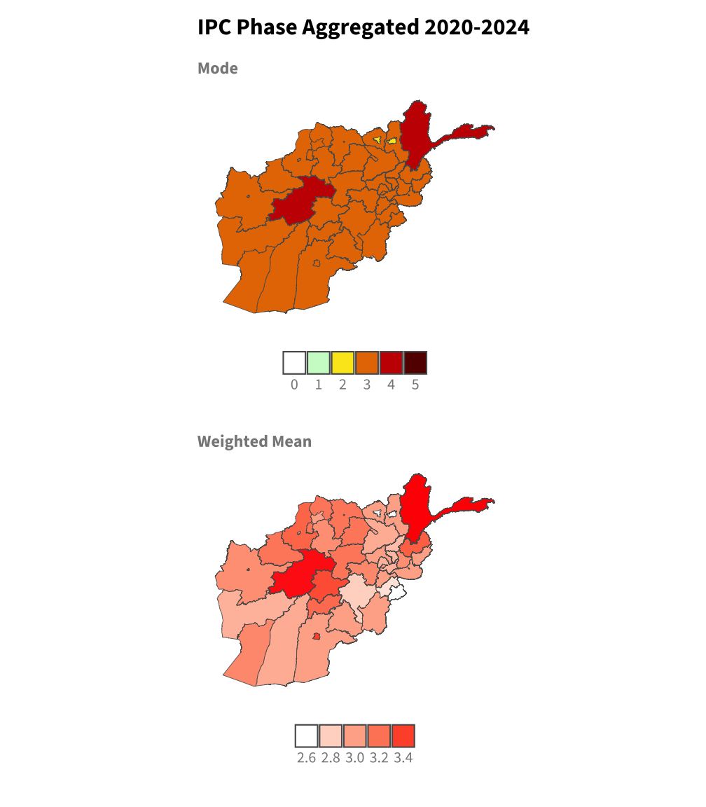
Finally we attempt to aggregate recent years by two methods as an attempt to try to understand where certain areas could be more vulnerable due to accumulated food insecurity stress over the recent years.

Code

mode <- function(codes) {
    which.max(tabulate(codes))
}

gdf_areas_filt_summarised <- gdf_areas_filt |>
    mutate(
        # go back to numeric
        overall_phase = as.numeric(overall_phase),
        yr = year(analysis_period_start),
        weights = case_when(
            yr == 2020 ~ 0.1,
            yr == 2021 ~ 0.15,
            yr == 2022 ~ 0.2,
            yr == 2023 ~ 0.25,
            yr == 2024 ~ 0.3
        )
    ) |>
    group_by(
        # area_id,
        area_name
    ) |>
    summarise(
        overall_phase_mean = mean(overall_phase, na.rm = T),
        overall_phase_median = median(overall_phase, na.rm = T),
        overall_phase_mode = mode(overall_phase),
        overall_phase_mean_weighted = weighted.mean(as.numeric(overall_phase), weights, na.rm = T),
        .groups = "drop"
    ) |>
    mutate(
        overall_phase_mode = fct_relevel(fct_expand(as_factor(overall_phase_mode), "0", "1", "2", "3", "4", "5"), "0", "1", "2", "3", "4", "5")
    )



p_ipc_mode <- ggplot() +
    geom_sf(
        data = gdf_areas_filt_summarised,
        aes(
            fill = overall_phase_mode
        ), show.legend = c(fill = TRUE)
    ) +
    scale_fill_manual(
        values = ipc_fill_pal,
        drop = FALSE
    ) +
    guides(
        fill = guide_legend(
            label.position = "bottom",
            nrow = 1, byrow = TRUE
        )
    ) +
    labs(
        subtitle = "Mode"
    ) +
    theme(
        legend.title = element_blank(),
        axis.text = element_blank(),
        panel.grid = element_blank(),
        axis.line.x.bottom = element_blank(),
        legend.key.spacing = unit(0, "cm"),
        legend.text = element_text(margin = margin(t = 3))
    )


p_ipc_weighted_mean <- ggplot() +
    geom_sf(
        data = gdf_areas_filt_summarised,
        aes(
            fill = overall_phase_mean_weighted
        ),
        show.legend = c(fill = TRUE)
    ) +
    scale_fill_gradient(
        low = "white", high = "red"
    ) +
    guides(
        fill = guide_legend(
            label.position = "bottom",
            nrow = 1, byrow = TRUE
        )
    ) +
    labs(
        subtitle = "Weighted Mean"
    ) +
    theme(
        legend.title = element_blank(),
        axis.text = element_blank(),
        panel.grid = element_blank(),
        axis.line.x.bottom = element_blank(),
        legend.key.spacing = unit(0, "cm"),
        legend.text = element_text(margin = margin(t = 3))
    )



p_ipc_mode +
    p_ipc_weighted_mean +
    plot_layout(
        nrow = 2, ncol = 1
    ) +
    plot_annotation(
        title = "IPC Phase Aggregated 2020-2024",
    )