8  Composite Indicator - Optimization Study

8.1 Intro

In this document we explore a method to find optimal weight sets. We create several parameter sets based on promising indicators as explored in the previous chapter. We then run an optimization procedure via a constrained grid search, iterating over all feasible weight combinations at 5% intervals to:

  1. maximize prediction accuracy/performance of end-of-season ASI
  2. minimize final variance across selected weights.

This optimization was largely done as a proof of concept to evaluate whether or not an optimal weight set could be created that adds value to a much simpler model that just looks at one indicator (ASI).

8.1.1 Key take-aways

We obtained satisfactory and value-adding results from all parameter combination sets. Therefore, a parameter set can be selected based on contextual criteria rather than marginal performance differences. Therefore the parameters set containing ERA5 Snow Cover rather than MODIS NDSI was selected to :

1.) allow a longer period of historical analysis: 1984 (start of ASI) rather than 2001 start of MODIS, 2.) remove complications that could arise in due to cloud interference in MODIS data set.

Code
aoi_adm1 <- c(
  "Takhar",
  # "Badakhshan",
  # "Badghis",
  "Sar-e-Pul" ,
  "Faryab"
  )

label_parameters <- function(df){
  df |>
    mutate(
     parameter_label = case_when(
      str_detect(parameter, "era5_land_volumetric_soil")~ "Soil Moisture (ERA5)",
      str_detect(parameter,"NDSI")~"NDSI",
      str_detect(parameter,"asi")~"ASI",
      str_detect(parameter,"vhi")~"VHI",

      str_detect(parameter,"cumu_chirps_precipitation_sum")~"Precip cumu (CHIRPS) ",
      str_detect(parameter,"chirps_precipitation_sum")~"Precip (CHIRPS)",
      str_detect(parameter,"cumu_era5_land_total_precipitation_sum")~"Precip cumu (ERA)",
      str_detect(parameter,"era5_land_total_precipitation_sum")~"Precip (ERA)",
      str_detect(parameter,"mean_2m_air_temperature")~"Temp (ERA)",
      str_detect(parameter,"era5_land_snow_depth_water_equivalent")~"SDWE (ERA5)",
      str_detect(parameter,"era5_land_snow_cover")~"Snow Cover (ERA5)",
      str_detect(parameter,"era5_land_snowmelt_sum")~"Snow Melt (ERA5)",

      str_detect(parameter,"runoff_max")~"Runoff max (ERA5)",
      str_detect(parameter,"runoff_sum")~"Runoff sum (ERA5)",
      str_detect(parameter,"SWE_inst")~"SWE (FLDAS)",

      .default = parameter
    )
    )
}
Code
SEASON_OF_INTEREST <- c(3,4,5)
# LATEST_SEASON_PREDICTABLE <-  c(3,4)

box::use(
  ../R/blob_connect,
  ../R/utils,
  seas5 = ../R/seas5_utils,
  loaders = ../R/load_funcs,
  dplyr[...],
  tidyr[...],
  stringr[...],
  glue[...],
  janitor[...],
  yardstick[...],
  ggplot2[...],
  gghdx[...],
  ggrepel[...],
  glue[...],
  lubridate[...],
  sf[...],
  readr[...],
  purrr[...],
  patchwork[...],
  cumulus
)

gghdx()
Code
df_compiled_indicators <- cumulus$blob_read(
  container = "projects",
  name = "ds-aa-afg-drought/processed/vector/df_all_combined_indicators_v2.parquet"
)

df_env_model <-
  df_compiled_indicators |>
  # df_env_compare |>
    select(
    date,
    yr_season,
    pub_mo_date,
    pub_mo_label,
    adm1_name,
    parameter,
    value
    ) |>
  filter(
    # these parameters are just a bit of noise
    !parameter %in% c("NDSI_Snow_Cover_min","NDSI_Snow_Cover_max","era5_land_runoff_max"),
    # these were consolidated into the average of all 4 soil moisture layers
    !str_detect(parameter,"era5_land_volumetric_soil_water_layer_\\d"),
    # already have these from ERA land up to 2024 rather than 2020
    !(parameter %in% c("total_precipitation","mean_2m_air_temperature"))

  )

# just some manual inspectino stuff here
df_env_model |>
  filter(str_detect(parameter,"^asi|^vhi")) |>
  group_by(parameter, pub_mo_label) |>
  count() |>
  pivot_wider(names_from=pub_mo_label, values_from = n)

date_ranges <- df_env_model |>
  group_by(parameter) |>
  summarise(
    start = min(pub_mo_date),
    end = max(pub_mo_date)
  )

8.1.2 Weighting Functons

Code
#' create_weight_grid
#' @description
#' function to create valid weight sets in long data.frame that can be
#' iterated through
#' @param x
#' @param wt_vals
#'
#' @returns
#' @export
#'
#' @examples
#' params_set_gte_1984 <- c(
#'   "era5_land_soil_moisture_1m",
#'   "cumu_era5_land_total_precipitation_sum",
#'   "vhi",
#'   "era5_land_snow_cover", # toying w/ adding this or not
#'   "asi"
#'   )
#' weight_combos <- create_weight_grid(params_set_gte_1984,wt_vals = c(0,seq(0.1, 1, by = 0.1)))

create_weight_grid <- function(x,wt_vals){

  df <- map(x,\(xt){
    tibble(
      !!sym(xt) :=wt_vals
    )
  }
  )|>
    list_cbind()

  df_expanded <- expand_grid(!!!df)

  df_valid_combinations <- df_expanded[rowSums(df_expanded) == 1, ]

    df_valid_combinations |>
      mutate(
        wt_id = row_number()
      ) |>
      pivot_longer(
        -wt_id, names_to = "parameter", values_to ="weight"
      )
}


#' Title
#'
#' @param df
#' @param params_included
#' @param earliest_year
#'
#' @returns
#' @export
#'
#' @examples
#' df_env_model |>
#'   normalize_to_z(params_included = l_params$gte1984,earliest_year = 1984)

normalize_to_z <- function(df,params_included, earliest_year){
      df |>
        filter(
          year(yr_season)>=earliest_year
        ) |>
        mutate(
        pub_mo_label = as.character(pub_mo_label)
      ) |>
      filter(
        parameter %in% params_included,
        pub_mo_label %in% c(month.abb[4:6])
      ) |>
      group_by(
        pub_mo_label, adm1_name, parameter
      ) |>
      mutate(
        zscore = scale(value,center=T,scale=T)[,1],
        zscore = ifelse(parameter != "asi",zscore*-1,zscore)
      )  |>
      ungroup()
}

#' Title
#'
#' @param df
#'
#' @returns
#' @export
#'
#' @examples
#' df_env_model |>
#'   normalize_to_z(params_included = l_params$gte2000,earliest_year = 2001) |>
#'   extract_truth_set()

extract_truth_set <- function(df){
  df |>
    filter(
      month(pub_mo_date)==6,
      parameter == "asi"
    ) |>
    select(
      yr_season, adm1_name, value,zscore_asi_Jun=zscore
    ) |>
    distinct()
}

#' Title
#'
#' @param df
#' @param params_included
#'
#' @returns
#' @export
#'
#' @examples
summarise_z <- function(
    df,
    params_included,
    weight_values
    ){

  df_weight_grid <- create_weight_grid(x = params_included, wt_vals = weight_values)

  df_filt <- df |>
    filter(
      parameter %in% params_included
    )
  split(df_filt,df_filt$pub_mo_label) |>
    map(\(dft){

      split(
        df_weight_grid,
        df_weight_grid$wt_id
      ) |>
        map(
          \(dft_w){

            dft_weighted <- dft |>
              left_join(
                dft_w, by = "parameter"
              )
            dft_summarised <- dft_weighted |>
              group_by(
                yr_season ,
                pub_mo_label,
                adm1_name,
                pub_mo_date,wt_id
              ) |>
              summarise(
                zscore = weighted.mean(zscore,w=weight,na.rm=T)
                ,.groups="drop"
              ) |>
              mutate(
                wt_set = list(dft_w)
              )
          }
        ) |>
        list_rbind()
    }
    ) |>
    list_rbind()

}


#' Title
#'
#' @param df
#' @param params_included
#' @param earliest_year
#' @param rp
#'
#' @returns
#' @export
#'
#' @examples
weighted_classify <- function(df,
                              params_included,
                              earliest_year,
                              rp=3,
                              weight_values ){
  df_normalized <- df |>
    normalize_to_z(
      params_included = params_included,
      earliest_year = earliest_year
    )

  df_truth <- df_normalized |>
    extract_truth_set()

  df_z_weighted <- df_normalized |>
    summarise_z(params_included = params_included,weight_values= weight_values)

   df_z_weighted |>
      left_join(
        df_truth |>
          select(-value)
      ) |>
      utils$threshold_var(
        var= "zscore",
        by = c("pub_mo_label","adm1_name","wt_id"),
        rp_threshold = rp
      ) |>
      utils$threshold_var(
        var= "zscore_asi_Jun",
        by = c("pub_mo_label","adm1_name","wt_id"),
        rp_threshold = rp
      ) |>
      arrange(adm1_name, yr_season,wt_id) |>
      ungroup()

}

single_indicator_performance <- function(df, parameter,earliest_year,rp){
  df_normalized <- df |>
    normalize_to_z(
      params_included = parameter,
      earliest_year = earliest_year
    )

  df_truth <- df_normalized |>
    extract_truth_set()


  df_classified <- df_normalized |>
    left_join(
      df_truth |>
        select(-value)
    ) |>
    utils$threshold_var(
      var= "zscore",
      by = c("pub_mo_label","adm1_name"),
      rp_threshold = rp
    ) |>
    utils$threshold_var(
      var= "zscore_asi_Jun",
      by = c("pub_mo_label","adm1_name"),
      rp_threshold = rp
    ) |>
    arrange(adm1_name, yr_season) |>
    ungroup()
  summarise_performance(df_classified,by = c("pub_mo_label","adm1_name"))
}
#' Title
#'
#' @param df
#' @param by
#'
#' @returns
#' @export
#'
#' @examples
summarise_performance <-  function(
    df,
    by=c("pub_mo_label","adm1_name","wt_id","wt_set"),
    parameter_subset = NULL
    ){
  if(!is.null(parameter_subset)){
    df |>
      filter(
        parameter %in% parameter_subset
      )
  }
  df |>
    mutate(
      across(ends_with("_flag"),\(x) factor(x,levels = c("TRUE","FALSE")))
    ) |>
    group_by(
      across({{by}})
    ) |>
    f_meas(zscore_asi_Jun_flag, zscore_flag, estimator= "binary",event_level = "first") |>
    ungroup()

}

#' Title
#'
#' @param df
#'
#' @returns
#' @export
#'
#' @examples
top_performance_per_moment <- function(df,n=1){
  # df=  ldf_perf_all_models$gte1984,n=1
  df_max <- df |>
    group_by(pub_mo_label, wt_id) |>
    summarise(
      avg_estimate = mean(.estimate)
    ) |>
    slice_max(
      order_by = avg_estimate,
      n= n
    )|>
    ungroup()

  inner_join(
    df_max,
    select(df,
           any_of(c("adm1_name","pub_mo_label", "wt_id", "wt_set",".estimate","asi_f1"))
           ),
    by = c("pub_mo_label","wt_id")
  )
}

#' Title
#'
#' @param df
#'
#' @returns
#' @export
#'
#' @examples
plot_optimal_compositions <-  function(df, label_plot = F, pal){

  df_labelled <- df|>
    select(
      pub_mo_label,adm1_name,wt_set,avg_estimate,.estimate
    ) |>
    unnest(wt_set) |>
    utils$label_parameters() |>
    mutate(
      p_label = glue(
      "id: {wt_id}
      f1: {scales::label_number(accuracy =0.001)(.estimate)}
      avg f1: {scales::label_number(accuracy =0.001)(avg_estimate)}"
      ),
      weight_pct_label = scales::percent(weight,accuracy = 1, trim = FALSE),
    )

  p <- df_labelled |>
    group_by(pub_mo_label, adm1_name) |>
    mutate(
      pub_mo_facet = factor(pub_mo_label,levels= c("Apr","May","Jun")),
      id = dense_rank(wt_id)
    ) |>
    ungroup() |>
    ggplot(
      aes(x= id, y= weight,fill = parameter_label)
    )+
    geom_bar(
      stat= "identity", color = "black"
    )+

    scale_fill_manual(values=pal)+
    facet_grid(cols= vars(pub_mo_facet),
               rows = vars(adm1_name)
               ,scales="free")+
    labs(
      x = "Different indicator weightings"

    )+
    scale_y_continuous(labels=scales::label_percent())+
    theme(
      legend.title = element_blank(),
      axis.text.x = element_blank()
    )
  if(label_plot){
    # df <- ldf_tops2$gte1984
    df |>
      mutate(
        p_label = glue("{wt_id}: {scales::label_number(accuracy =0.01)(avg_estimate)}")
      )
    p <- p +
      # composition plot
      geom_text(
        aes(x= id, y= weight, label = weight_pct_label),
        position = position_stack(vjust = 0.5), color ="black"
      )+
      # wt plot
      geom_label(aes(x= id, y= 1.1, label = p_label), color ="black",fill="beige",alpha=0.4)+
      # theme(
      #   panel.spacing.y = unit(4, "lines")
      # )+
      expand_limits(y = 1.2)
  }
  p
}


#' Title
#' helper func to find weight ids that are simple and optimal
#' not a perfect solution, but gets us 90% there.
#' @param df
#'
#' @returns
#' @export
#'
#' @examples
plot_low_var_optimal <-  function(df,
                                  pal,
                                  label_wt_id =T){


  dfp <- df|>
    select(
      pub_mo_label, wt_set
    ) |>
    unnest(wt_set) |>
    group_by(
      pub_mo_label,wt_id
    ) |>
    mutate(
      sd = sd(weight)

    ) |>
    group_by(pub_mo_label) |>
    slice_min(sd) |>
    group_by(pub_mo_label) |>
    mutate(
      pub_mo_facet = factor(pub_mo_label,levels= c("Apr","May","Jun")),
      id = dense_rank(wt_id)
    ) |>
    ungroup() |>
    utils$label_parameters()

  p <- dfp |>
    distinct() |>
    mutate(
      weight_pct_label = scales::percent(weight,accuracy = 1, trim = FALSE),
      weight_id_label = glue("weight id: {wt_id}")

    ) |>
    filter(pub_mo_label!= "Jun") |>
    ggplot(
      aes(
        x= id,
        y= weight,
        fill = parameter_label
      ),
      position = position_stack(vjust = 0.5)
    )+
    geom_bar(
      stat= "identity", color = "black"
    )+

    geom_text(aes(x= id, y= weight, label = weight_pct_label),
              position = position_stack(vjust = 0.5), color ="black")+
    scale_fill_manual(values=pal) +
    scale_y_continuous(labels =scales::label_percent())+
    facet_grid(cols= vars(pub_mo_facet)
               ,scales="free")+
    labs(
      # title = "May publication weight combos that give avg 0.90 f1"
    )
  if(label_wt_id){
    p <- p +
      geom_text(
        aes(
          x= id+.25,
          y= 0.5,
          label = weight_id_label
          ), color ="black"
      )
  }
  p
}


#' Title
#'
#' @param df
#' @param param_simple
#'
#' @returns
#' @export
#'
#' @examples
get_simple_weight_id <- function(df,param_simple){
    df |>
    select(wt_set) |>
    unnest(wt_set) |>
    distinct() |>
    filter(
      parameter == param_simple ,
      weight == 1
    ) |>
    pull(wt_id) |>
    unique()

}
#' Title
#' @description
#' After plotting different optimal weight combinations you might want to compare specific
#' weighting compositions to a simpler model (i.e ASI). So this allows you to plug in the
#' weight ids for both april and may as well as `param_simple` which has always been ASI up to
#' this point in analysis. The output data.frame is interesting for plotting.
#'
#' @param df
#' @param wt_id_apr
#' @param wt_id_may
#' @param param_simple
#'
#' @returns
#' @export
#'
#' @examples
compare_to_simple_model <- function(df,wt_id_apr, wt_id_may,param_simple){
  simple_model_id <-get_simple_weight_id(df= df, param_simple = param_simple)

    df_chosen <- df |>
      summarise_performance() |>
      filter(
        (pub_mo_label == "Apr" & wt_id==wt_id_apr)|
        (pub_mo_label == "May" & wt_id==wt_id_may)|
        wt_id == simple_model_id

      ) |>
      filter(pub_mo_label != "Jun")

    df_simple <- df_chosen |>
      filter(
        wt_id == simple_model_id
      )
    anti_join(df_chosen,df_simple) |>
      left_join(
        df_simple |>
          select(
            pub_mo_label,adm1_name,
            estimate_simple =.estimate),
        by = c("pub_mo_label","adm1_name")
      )

}
8.2 Parameter Sets

We create 4 parameter combination sets.

Code
# setup as many sets of parameters as we want
# subequent code will iterate through each parameter set

params_set_gte_2001 <- c(
  "era5_land_soil_moisture_1m",
  "cumu_era5_land_total_precipitation_sum",
  "NDSI_Snow_Cover_mean",
  "vhi",
  "asi"
)

# and one that takes data going back to 1984
params_set_gte_1984 <- c(
  "era5_land_soil_moisture_1m",
  "cumu_era5_land_total_precipitation_sum",
  "vhi",
  "era5_land_snow_cover", # toying w/ adding this or not
  "asi"
)
params_set_gte_1984_no_snow <- c(
  "era5_land_soil_moisture_1m",
  "cumu_era5_land_total_precipitation_sum",
  "vhi",
  "asi"
)

params_set_gte_1984_w_mixed_forecast_obs <- c(
  "era5_land_soil_moisture_1m",
  "cumu_era5_land_total_precipitation_sum",
  "vhi",
  "mam_mixed_seas_observed",
    "era5_land_snow_cover",
  "asi"
)

l_params <- list(
  "gte2001"= params_set_gte_2001,
  "gte1984" = params_set_gte_1984,
  "gte_1984_no_snow" = params_set_gte_1984_no_snow,
  "gte_1984_w_mixed_forecast_obs" = params_set_gte_1984_w_mixed_forecast_obs
)

# cram those into table!
df_parameter_configs <- tibble(
  param_set_id = names(l_params),
  parameter_sets = l_params,
  earliest_year =parse_number(param_set_id)
)

The different combinations sets are composed of various combinations of era5_land_soil_moisture_1m, cumu_era5_land_total_precipitation_sum, NDSI_Snow_Cover_mean, vhi, asi, era5_land_snow_cover, and mam_mixed_seas_observed

The key distinctions are:

  1. whether or no to include snow. And if using snow, whether to use MODIS NDSI or ERA5 Snow Cover.
  2. After various iterations with working group mixed observational-forecast indicator was created and included in one of the final sets.

8.2.1 Weight implementation

Code
# run weighting and aggregations

# For each paramter set (i.e gte1984, gte_1984_no_snow, gte2001) this returns
# 1. a historical data set per model composition
# 2. an assessment of f1 performance of each model set measuring against
# reference framework of just using ASI

# this takes approx 10 minutes to run on my computer. There are many millions
# of rows .. could save as a file, but it will take a long time even load
# from the blob.

system.time(
  ldf_perf <- pmap(
  list(
    df_parameter_configs$param_set_id,
    df_parameter_configs$parameter_sets,
    df_parameter_configs$earliest_year
    ),
  \(id,params, start_yr){

    # cat("reclassifying\n")
    df_all_weights_flagged <- weighted_classify(
      df = df_env_model,
      earliest_year = start_yr,
      params_included = unlist(params),
      weight_values = seq(0,1,by =0.05),
      rp=3
    )

    df_asi_perf <-  single_indicator_performance(
      df_env_model,
      parameter = "asi",
      earliest_year = start_yr,
      rp=3
    )

    df_perf <- df_all_weights_flagged |>
      summarise_performance() |>
       left_join(
        df_asi_perf |>
          rename(asi_f1 = .estimate)
        )

    l_ret <- list(
      ALL_MODELS = df_perf,
      HISTORICAL_WEIGHTED = df_all_weights_flagged
    )
    l_ret
  }
)
)

ldf_perf <- set_names(ldf_perf,df_parameter_configs$param_set_id)

# extract historical data.frame sets
ldf_historical <-  ldf_perf |>
  map("HISTORICAL_WEIGHTED")

ldf_perf_all_models <- ldf_perf |>
  map("ALL_MODELS")

ldf_top3 <- ldf_perf_all_models |>
  map(\ (dft){
    dft |>
      top_performance_per_moment(n=3)
  })

8.3 Weighting results

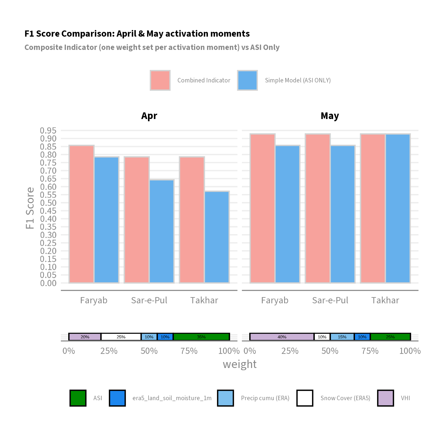
To evaluate value-add of optimal weight sets, we compare them with a simpler indicator model that only utilizes the ASI for the current month/activation model (a strongly perfoming single indicator). For the sake of brevity simplicity/we will not plot all weight sets explored in the rendered document, but rather display results as a proof of concept.

8.3.1 Weight Set A:

below we show a comparison of F1 scores for the optimal indicator weighting found in a weight set of ASI, VHI, ERA5 Snow, ERA5 Soil Moisture, & ERA5 Cumulative precipitation.

We see significant gains in performance across provinces and months when compared to a simple ASI model.

Code
ldf_top3$gte1984 |>
  filter(pub_mo_label!="Jun") |>
  group_by(pub_mo_label, adm1_name) |>
  slice_max(avg_estimate,with_ties = F) |>
  # left_join(df_asi_performance |> rename(asi_f1 = .estimate)) |>
  pivot_longer (cols = c(".estimate","asi_f1")) |>
  mutate(
    indicator_label = ifelse(name == ".estimate", "Combined Indicator","Simple Indicator (ASI)" )
  ) |>
  ggplot(
    aes(x = adm1_name, y =value, fill = indicator_label)
  )+
  geom_bar(stat="identity", position = "dodge")+
  scale_fill_manual(
    values = c("Combined Indicator"=hdx_hex("tomato-light"), "Simple Indicator (ASI)"=hdx_hex("sapphire-light"))
  )+
  facet_wrap(~pub_mo_label)+
  scale_y_continuous(
    breaks = seq(0,1,by = 0.05)
  )+
  labs(
    title = "F1 Score Comparison: Composite Indicator vs ASI Only",
    subtitle= "Analysis 1984-present (including ERA5 snow)",
    caption= "Composite indicator contains optimal weighted aggregations of Snow Cover (ERA5), Soil Moisture (ERA5), ASI (FAO), VHI (FAO), and cumulative precipitation (ERA 5)",
    y= "F1 Score"
  )+
  theme(
    legend.title=element_blank(),
    axis.title.x = element_blank()
  )

pal_indicator_composition <-  c("ASI"="green4",
                                "VHI"="#CAB2D6",
                                "NDSI"= "#6A3D9A",
                                "Precip cumu (ERA)"= "skyblue2",
                                "era5_land_soil_moisture_1m"= "dodgerblue2",
                                "Snow Cover (ERA5)"= "white")


p_optimal_low_variance_weights <- plot_low_var_optimal(
  ldf_top3$gte1984,
  pal = pal_indicator_composition,
  label_wt_id = F
)+
  coord_flip()
Code
df_compare <- compare_to_simple_model(
  ldf_historical$gte1984,
  wt_id_apr = 3316,#379 -- was optimal when did weight by 0.1 #14 is optimal
  wt_id_may = 3490, #142 & 84 are optimal for May, but dont include soil moisture
  param_simple = "asi"
  )

p_optimal_chosen_compared_to_asi <- df_compare |>
  pivot_longer(
    cols = c(".estimate","estimate_simple")
    ) |>
  mutate(
    name = ifelse(str_detect(name,".estimate"), "Combined Indicator","Simple Model (ASI ONLY)")
  ) |>
  ggplot(
    aes(x= adm1_name,y= value, fill = name )
  ) +
  geom_bar(stat= "identity", position = "dodge", color = "lightgrey") +
    scale_y_continuous(
    breaks = seq(0,1,by = 0.05)
  )+
  scale_fill_manual(
    values = c("Combined Indicator"=hdx_hex("tomato-light"), "Simple Model (ASI ONLY)"=hdx_hex("sapphire-light"))
  )+
  labs(
    title = "F1 Score Comparison: April & May activation moments",
    subtitle= "Composite Indicator (one weight set per activation moment) vs ASI Only",
    caption= "Composite indicator created via weighted aggregation of z-scores of cumulative rainfall (ERA5), snow cover (NDSI), Soil Moisture (ERA5), VHI (FAO), ASI (FAO)",
    y= "F1 Score"
  )+
  facet_wrap(~pub_mo_label)+
  theme(
    legend.title=element_blank(),
    axis.title.x = element_blank()
  )

p_optimal_chosen_compared_to_asi +
  theme(
    text = element_text(size= 24),
    plot.caption = element_blank(),
    legend.position = "top",
    plot.title = element_text(size= 24),
    plot.subtitle = element_text(size= 20),
    legend.text = element_text(size=16)
  )+
  p_optimal_low_variance_weights+
  theme(
    text = element_text(size= 24),
    legend.text = element_text(size= 16),
    legend.key.size = unit(0.5, "cm"),
    axis.title.y= element_blank(),
    axis.text.y= element_blank(),
    strip.text = element_blank(),
    legend.title = element_blank()
  )+
  plot_layout(nrow=2,heights = c(1,0.05))

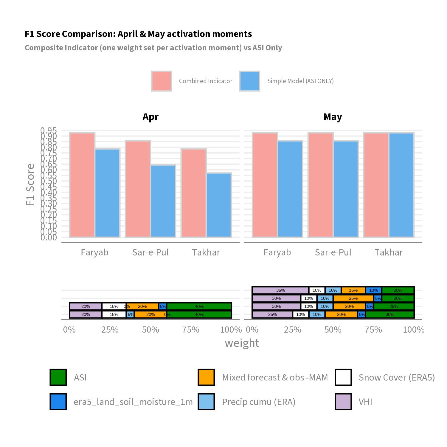
8.3.2 Weight Set B:

Weight set B utilizes the same indicators as Weight Set A, but includes the Mixed forecast and observational indicator. We also see a value add over the simple ASI indicator model. Additionally we see an increase in F1 scores for the month of April in 2 out of 3 of the provinces. This hints that the mixed observational forecast may be a useful indicator to keep included.

Code
pal_indicator_composition2 <-  c("ASI"="green4",
                                "VHI"="#CAB2D6",
                                "NDSI"= "#6A3D9A",
                                "Precip cumu (ERA)"= "skyblue2",
                                "era5_land_soil_moisture_1m"= "dodgerblue2",
                                "Snow Cover (ERA5)"= "white",
                                "Mixed forecast & obs -MAM"= "orange")

ldf_top3$gte_1984_w_mixed_forecast_obs |>
  filter(pub_mo_label!="Jun") |>
  group_by(pub_mo_label, adm1_name) |>
  slice_max(avg_estimate,with_ties = F) |>
  # left_join(df_asi_performance |> rename(asi_f1 = .estimate)) |>
  pivot_longer (cols = c(".estimate","asi_f1")) |>
  mutate(
    indicator_label = ifelse(name == ".estimate", "Combined Indicator","Simple Indicator (ASI)" )
  ) |>
  ggplot(
    aes(x = adm1_name, y =value, fill = indicator_label)
  )+
  geom_bar(stat="identity", position = "dodge")+
  scale_fill_manual(
    values = c("Combined Indicator"=hdx_hex("tomato-light"), "Simple Indicator (ASI)"=hdx_hex("sapphire-light"))
  )+
  facet_wrap(~pub_mo_label)+
  scale_y_continuous(
    breaks = seq(0,1,by = 0.05)
  )+
  labs(
    title = "F1 Score Comparison: Composite Indicator vs ASI Only",
    subtitle= "Analysis 1984-present (including ERA5 snow)",
    caption= "Composite indicator contains optimal weighted aggregations of Snow Cover (ERA5), Soil Moisture (ERA5), ASI (FAO), VHI (FAO), and cumulative precipitation (ERA 5)",
    y= "F1 Score"
  )+
  theme(
    legend.title=element_blank(),
    axis.title.x = element_blank()
  )
Code
# this takes a minute

df_compare_gte_1984_w_mixed_forecast_obs <- compare_to_simple_model(
  ldf_historical$gte_1984_w_mixed_forecast_obs,
  wt_id_apr = 9834,
  wt_id_may = 12297, #142 & 84 are optimal for May, but dont include soil moisture
  param_simple = "asi"
  )


p_comparison_1984_w_mixed_forecast_obs <- df_compare_gte_1984_w_mixed_forecast_obs |>
  pivot_longer(cols = c(".estimate","estimate_simple")) |>
  mutate(
    name = ifelse(str_detect(name,".estimate"), "Combined Indicator","Simple Model (ASI ONLY)")
  ) |>
  ggplot(
    aes(x= adm1_name,y= value, fill = name )
  ) +
  geom_bar(stat= "identity", position = "dodge", color = "lightgrey") +
    scale_y_continuous(
    breaks = seq(0,1,by = 0.05)
  )+
  scale_fill_manual(
    values = c("Combined Indicator"=hdx_hex("tomato-light"), "Simple Model (ASI ONLY)"=hdx_hex("sapphire-light"))
  )+
  labs(
    title = "F1 Score Comparison: April & May activation moments",
    subtitle= "Composite Indicator (one weight set per activation moment) vs ASI Only",
    caption= "Composite indicator created via weighted aggregation of z-scores of cumulative rainfall (ERA5), snow cover (NDSI), Soil Moisture (ERA5), VHI (FAO), ASI (FAO)",
    y= "F1 Score"
  )+
  facet_wrap(~pub_mo_label)+
  theme(
    legend.title=element_blank(),
    axis.title.x = element_blank()
  )

p_comparison_1984_w_mixed_forecast_obs +
  theme(
    text = element_text(size= 24),
    plot.caption = element_blank(),
    legend.position = "top",
    plot.title = element_text(size= 24),
    plot.subtitle = element_text(size= 20),
    legend.text = element_text(size=16)
  )+
  p_optimal_low_variance_weights_w_mixed+
  theme(
    text = element_text(size= 24),
    axis.title.y= element_blank(),
    axis.text.y= element_blank(),
    strip.text = element_blank(),
    legend.title = element_blank(),
    legend.key.size = unit(0.5, "cm"),
    legend.text = element_text(size=16)
  )+
  plot_layout(nrow=2,heights = c(0.5,0.15))+
  theme(
    theme(plot.margin = c(0,0,0,0))
  )