Code
box::use(
    dplyr[...],
    tidyr[...],
    ggplot2[...],
    gghdx[...],
    cumulus[...],
    purrr[...],
    glue[glue],
    tibble[tibble],
    .. / R / utils[rp_empirical]
)

library(tidymodels)
library(gt)
gghdx()This chapter proposes a two-stage trigger for the 2026 anticipatory action framework. The idea is to combine two independent signals at different lead times using OR logic:
A year triggers if either signal fires. This increases sensitivity (fewer missed droughts) at the cost of more frequent activation.
See ?sec-2026-trigger-modeling for CDI model derivation and validation.
box::use(
dplyr[...],
tidyr[...],
ggplot2[...],
gghdx[...],
cumulus[...],
purrr[...],
glue[glue],
tibble[tibble],
.. / R / utils[rp_empirical]
)
library(tidymodels)
library(gt)
gghdx()# Return period threshold for defining drought
RP_THRESHOLD <- 4
# Random seed
SEED <- 42
# Bootstrap resamples
N_BOOTSTRAP <- 30
# Feature set paths
FEATURE_PATHS <- list(
march = "ds-aa-afg-drought/processed/vector/2026_mar_pub_feature_set_v1.parquet",
april = "ds-aa-afg-drought/processed/vector/2026_april_pub_feature_set_v1.parquet"
)
# Variables to exclude from CDI model (same as ch12)
APRIL_EXCLUDE_VARS <- c("total_precipitation_sum", "seas5 Apr", "seas5 May")# Load feature sets
df_mar_raw <- blob_read(name = FEATURE_PATHS$march, container = "projects")
df_apr_raw <- blob_read(name = FEATURE_PATHS$april, container = "projects")
# Prepare modeling data with empirical RP thresholding
prepare_model_data <- function(df, rp_threshold = RP_THRESHOLD) {
df |>
filter(!is.na(outcome_asi_zscore)) |>
arrange(desc(outcome_asi_zscore)) |>
mutate(
rank = row_number(),
q_rank = rank / (n() + 1),
rp_emp = 1 / q_rank,
drought = factor(
if_else(rp_emp >= rp_threshold, "yes", "no"),
levels = c("yes", "no")
)
) |>
select(-outcome_asi_zscore, -rank, -q_rank, -rp_emp,
-starts_with("adm0_name"), -pub_date, -timestep)
}
df_mar <- prepare_model_data(df_mar_raw)
df_apr <- prepare_model_data(df_apr_raw)# Ridge specification
ridge_spec <- logistic_reg(penalty = tune(), mixture = 0) |>
set_engine("glmnet") |>
set_mode("classification")
# Recipe (exclude composite components + precip_cumsum, same as ch12)
ridge_recipe <- recipe(drought ~ ., data = df_apr) |>
step_rm(all_of(c("pub_year", APRIL_EXCLUDE_VARS, "precip_cumsum"))) |>
step_zv(all_predictors())
ridge_wf <- workflow() |>
add_recipe(ridge_recipe) |>
add_model(ridge_spec)
# Tune penalty
set.seed(SEED)
ridge_boots <- bootstraps(df_apr, times = N_BOOTSTRAP, strata = drought)
penalty_grid <- grid_regular(penalty(range = c(-4, 0)), levels = 30)
ridge_tune <- tune_grid(
ridge_wf,
resamples = ridge_boots,
grid = penalty_grid,
metrics = metric_set(roc_auc, f_meas),
control = control_grid(save_pred = TRUE)
)
best_penalty <- select_best(ridge_tune, metric = "f_meas")
final_ridge_fit <- fit(finalize_workflow(ridge_wf, best_penalty), data = df_apr)
# Extract CDI weights
coefs_ridge <- final_ridge_fit |>
extract_fit_parsnip() |>
tidy() |>
filter(term != "(Intercept)")
cdi_weights <- coefs_ridge |>
mutate(
weight = -estimate / sum(abs(estimate)),
contribution_pct = abs(weight) * 100
) |>
arrange(desc(contribution_pct)) |>
select(term, estimate, weight, contribution_pct)
# F1-optimized probability threshold → CDI threshold (same derivation as ch12)
prob_drought <- predict(final_ridge_fit, df_apr, type = "prob")$.pred_yes
thresholds <- seq(0.1, 0.9, by = 0.05)
best_prob_threshold <- map_dfr(thresholds, function(thresh) {
pred <- factor(if_else(prob_drought > thresh, "yes", "no"), levels = c("yes", "no"))
tibble(threshold = thresh, f1 = yardstick::f_meas_vec(df_apr$drought, pred))
}) |>
filter(f1 == max(f1, na.rm = TRUE)) |>
slice(1) |>
pull(threshold)formula_parts <- cdi_weights |>
arrange(desc(weight)) |>
mutate(
part = paste0(
if_else(row_number() == 1, "", " + "),
round(weight, 3), " × ", term
)
) |>
pull(part)
cat("**CDI Formula:**\n\n$$\\text{CDI} = ", paste(formula_parts, collapse = ""), "$$\n")CDI Formula:
\[\text{CDI} = 0.275 × mixed_fcast_obsv + 0.206 × asi + 0.205 × snow_cover + 0.192 × vhi + 0.121 × volumetric_soil_water_1m \]
# CDI calculation helper
calc_cdi <- function(data, weights_df) {
    cdi <- rep(0, nrow(data))
    for (i in seq_len(nrow(weights_df))) {
        feat <- weights_df$term[i]
        w <- weights_df$weight[i]
        if (feat %in% colnames(data)) {
            cdi <- cdi + w * data[[feat]]
        }
    }
    cdi
}

# Build historical record with both signals
df_historical <- tibble(
    year = df_apr$pub_year,
    drought_actual = df_apr$drought,
    cdi = calc_cdi(df_apr, cdi_weights),
    prob_drought = prob_drought,
    seas5_mam = df_mar$`seas5 Mar-Apr-May`
) |>
    mutate(
        cdi_rp = rp_empirical(cdi, direction = "-1"),
        seas5_rp = rp_empirical(seas5_mam, direction = "-1")
    )

# CDI threshold from F1-optimized probability (consistent with ch12)
cdi_threshold <- min(df_historical$cdi[df_historical$prob_drought > best_prob_threshold])
n_trigger_tuned <- sum(df_historical$prob_drought > best_prob_threshold)
rp_f1_equivalent <- round((nrow(df_historical) + 1) / n_trigger_tuned, 2)The heatmap below shows the effective return period of the combined two-stage trigger across all combinations of CDI and SEAS5 thresholds. OR logic means a year triggers if either signal exceeds its threshold.
rp_grid <- expand_grid(
    cdi_threshold = 3:7,
    seas5_threshold = 3:7
) |>
    pmap_dfr(function(cdi_threshold, seas5_threshold) {
        n_either <- df_historical |>
            filter(cdi_rp >= cdi_threshold | seas5_rp >= seas5_threshold) |>
            nrow()

        tibble(
            cdi_threshold = cdi_threshold,
            seas5_threshold = seas5_threshold,
            n_triggered = n_either,
            n_years = nrow(df_historical),
            rp_combined = if (n_either > 0) round(nrow(df_historical) / n_either, 1) else Inf
        )
})rp_grid |>
mutate(
rp_label = if_else(
is.infinite(rp_combined),
"never",
as.character(rp_combined)
),
rp_fill = if_else(
is.infinite(rp_combined),
max(rp_combined[is.finite(rp_combined)]) + 5,
rp_combined
),
target_zone = rp_combined >= 3 & rp_combined <= 5 & is.finite(rp_combined)
) |>
ggplot(aes(
x = factor(cdi_threshold),
y = factor(seas5_threshold),
fill = rp_fill
)) +
geom_tile(color = "white", linewidth = 1) +
geom_text(aes(label = rp_label), fontface = "bold", size = 4.5) +
geom_tile(
data = \(d) filter(d, target_zone),
aes(x = factor(cdi_threshold), y = factor(seas5_threshold)),
fill = NA, color = "black", linewidth = 1.5
) +
scale_fill_gradient2(
low = "tomato", mid = "khaki", high = "steelblue",
midpoint = 5,
name = "Combined\nRP (years)"
) +
labs(
title = "Combined Return Period: Two-Stage Trigger (OR Logic)",
subtitle = "Black border = RP 3\u20135 target zone",
x = "CDI Threshold (RP, years)",
y = "SEAS5 March Threshold (RP, years)"
) +
theme(panel.grid = element_blank())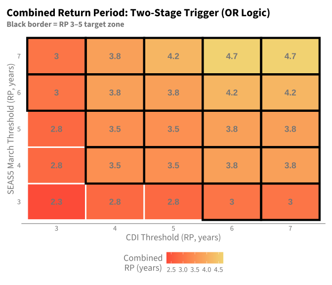
Interpretation: Lower-left cells (both thresholds lenient) fire frequently and have low combined RP. Upper-right cells (both thresholds strict) fire rarely. The RP 3–5 target zone (black border) identifies threshold pairs consistent with the program’s desired activation frequency. Because OR logic combines two signals, the combined RP is always less than or equal to the minimum of the individual RPs.
The zoomed view below uses finer increments (0.2) to show exactly where our proposed threshold sits. The black-bordered cell marks CDI ≈ RP 3.91 (F1-tuned) combined with SEAS5 RP 4 (best early:false ratio).
# Fine-grained RP breaks
rp_fine <- seq(3, 5, by = 0.2)

# Snap our tuned RP to nearest grid point
tuned_cdi_snap <- rp_fine[which.min(abs(rp_fine - rp_f1_equivalent))]

rp_grid_zoom <- expand_grid(
    cdi_threshold = rp_fine,
    seas5_threshold = rp_fine
) |>
    pmap_dfr(function(cdi_threshold, seas5_threshold) {
        n_either <- df_historical |>
            filter(cdi_rp >= cdi_threshold | seas5_rp >= seas5_threshold) |>
            nrow()

        tibble(
            cdi_threshold = cdi_threshold,
            seas5_threshold = seas5_threshold,
            n_triggered = n_either,
            n_years = nrow(df_historical),
            rp_combined = if (n_either > 0) round(nrow(df_historical) / n_either, 1) else Inf
        )
    })

rp_grid_zoom |>
    mutate(
        rp_label = if_else(
            is.infinite(rp_combined),
            "never",
            as.character(rp_combined)
        ),
        rp_fill = if_else(
            is.infinite(rp_combined),
            max(rp_combined[is.finite(rp_combined)]) + 5,
            rp_combined
        )
    ) |>
    ggplot(aes(
        x = factor(cdi_threshold),
        y = factor(seas5_threshold),
        fill = rp_fill
    )) +
    geom_tile(color = "white", linewidth = 0.5) +
    geom_text(aes(label = rp_label), fontface = "bold", size = 2.5) +
    # Highlight proposed threshold
    annotate("rect",
             xmin = which(rp_fine == tuned_cdi_snap) - 0.5,
             xmax = which(rp_fine == tuned_cdi_snap) + 0.5,
             ymin = which(rp_fine == 4) - 0.5,
             ymax = which(rp_fine == 4) + 0.5,
             fill = NA, color = "black", linewidth = 2) +
    scale_fill_gradient2(
        low = "tomato", mid = "khaki", high = "steelblue",
        midpoint = 5,
        name = "Combined\nRP (years)"
    ) +
    labs(
        title = "Zoomed: Combined Return Period (RP 3–5 range)",
        subtitle = glue("Black border = proposed threshold (CDI ≈ RP {rp_f1_equivalent}, SEAS5 RP 4)"),
        x = "CDI Threshold (RP, years)",
        y = "SEAS5 March Threshold (RP, years)"
    ) +
    theme(
        panel.grid = element_blank(),
        axis.text.x = element_text(size = 7, angle = 45, hjust = 1),
        axis.text.y = element_text(size = 7)
    )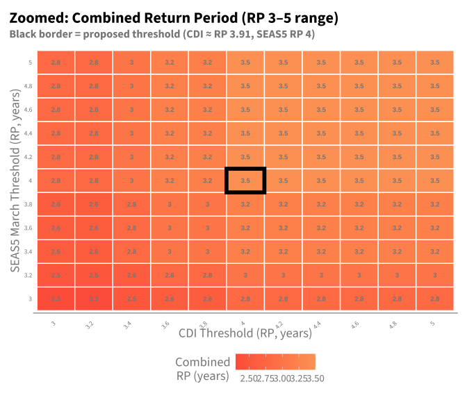
At CDI ≈ RP 3.91 and SEAS5 RP 4, the combined trigger has an effective return period of approximately 3.5 years — within the target RP 3–5 range for anticipatory action.
This section provides explicit, transparent calculations for the return periods used in the 2026 trigger system.
# CDI threshold and equivalent RP
n_cdi_fires <- sum(df_historical$cdi >= cdi_threshold)
cdi_rp_exact <- (nrow(df_historical) + 1) / n_cdi_fires

# SEAS5 thresholds (testing RP 4 and RP 6)
n_seas5_rp4_fires <- sum(df_historical$seas5_rp >= 4)
n_seas5_rp6_fires <- sum(df_historical$seas5_rp >= 6)

seas5_rp4_exact <- (nrow(df_historical) + 1) / n_seas5_rp4_fires
seas5_rp6_exact <- (nrow(df_historical) + 1) / n_seas5_rp6_fires

# Years where each fires
years_cdi_fires <- df_historical$year[df_historical$cdi >= cdi_threshold]
years_seas5_rp4_fires <- df_historical$year[df_historical$seas5_rp >= 4]
years_seas5_rp6_fires <- df_historical$year[df_historical$seas5_rp >= 6]

# Combined (OR logic)
years_combined_rp4 <- unique(c(years_cdi_fires, years_seas5_rp4_fires))
years_combined_rp6 <- unique(c(years_cdi_fires, years_seas5_rp6_fires))

n_combined_rp4 <- length(years_combined_rp4)
n_combined_rp6 <- length(years_combined_rp6)

combined_rp_rp4 <- round(nrow(df_historical) / n_combined_rp4, 2)
combined_rp_rp6 <- round(nrow(df_historical) / n_combined_rp6, 2)| Component | Threshold | Years Firing | Empirical RP |
|---|---|---|---|
| CDI (April) | F1-optimized | 11 of 42 | 3.91 years |
| SEAS5 (March) | RP ≥ 4 | 10 of 42 | 4.3 years |
| SEAS5 (March) | RP ≥ 6 | 7 of 42 | 6.14 years |
The combined trigger fires if either CDI OR SEAS5 exceeds its threshold. The combined RP is calculated as: \[ \text{Combined RP} = \frac{N_{\text{years}}}{\text{Years where (CDI fires) OR (SEAS5 fires)}} \]
cat("**Years where CDI fires:**\n\n")Years where CDI fires:
cat(paste(sort(years_cdi_fires), collapse = ", "), "\n\n")2000, 2001, 2004, 2006, 2008, 2011, 2018, 2021, 2022, 2023, 2025
cat("**Years where SEAS5 RP ≥ 4 fires:**\n\n")Years where SEAS5 RP ≥ 4 fires:
cat(paste(sort(years_seas5_rp4_fires), collapse = ", "), "\n\n")1985, 2000, 2001, 2004, 2006, 2008, 2010, 2018, 2021, 2023
cat("**Years where EITHER fires (union):**\n\n")Years where EITHER fires (union):
cat(paste(sort(years_combined_rp4), collapse = ", "), "\n\n")1985, 2000, 2001, 2004, 2006, 2008, 2010, 2011, 2018, 2021, 2022, 2023, 2025
cat(glue("**Calculation:** {nrow(df_historical)} years ÷ {n_combined_rp4} years triggered = **{combined_rp_rp4} year RP**\n"))Calculation: 42 years ÷ 13 years triggered = 3.23 year RP
cat("**Years where CDI fires:**\n\n")Years where CDI fires:
cat(paste(sort(years_cdi_fires), collapse = ", "), "\n\n")2000, 2001, 2004, 2006, 2008, 2011, 2018, 2021, 2022, 2023, 2025
cat("**Years where SEAS5 RP ≥ 6 fires:**\n\n")Years where SEAS5 RP ≥ 6 fires:
cat(paste(sort(years_seas5_rp6_fires), collapse = ", "), "\n\n")1985, 2000, 2001, 2004, 2006, 2008, 2018
cat("**Years where EITHER fires (union):**\n\n")Years where EITHER fires (union):
cat(paste(sort(years_combined_rp6), collapse = ", "), "\n\n")1985, 2000, 2001, 2004, 2006, 2008, 2011, 2018, 2021, 2022, 2023, 2025
cat(glue("**Calculation:** {nrow(df_historical)} years ÷ {n_combined_rp6} years triggered = **{combined_rp_rp6} year RP**\n"))Calculation: 42 years ÷ 12 years triggered = 3.5 year RP
tibble(
    `Trigger Configuration` = c(
        "CDI only (April)",
        "SEAS5 RP ≥ 4 only (March)",
        "SEAS5 RP ≥ 6 only (March)",
        "CDI OR SEAS5 RP ≥ 4",
        "CDI OR SEAS5 RP ≥ 6"
    ),
    `Years Triggered` = c(
        n_cdi_fires,
        n_seas5_rp4_fires,
        n_seas5_rp6_fires,
        n_combined_rp4,
        n_combined_rp6
    ),
    `Empirical RP` = c(
        round(cdi_rp_exact, 2),
        round(seas5_rp4_exact, 2),
        round(seas5_rp6_exact, 2),
        combined_rp_rp4,
        combined_rp_rp6
    )
) |>
    gt() |>
    tab_header(
        title = "Exact Return Period Calculations",
        subtitle = glue("Based on {nrow(df_historical)} years of historical data (1984-2025)")
    ) |>
    cols_label(
        `Trigger Configuration` = "Configuration",
        `Years Triggered` = "N Years Fired",
        `Empirical RP` = "RP (years)"
    ) |>
    tab_style(
        style = cell_fill(color = "#E8F5E9"),
        locations = cells_body(rows = `Trigger Configuration` == "CDI OR SEAS5 RP ≥ 6")
    ) |>
    tab_footnote(
        footnote = "Green row = recommended configuration",
        locations = cells_column_labels(columns = `Trigger Configuration`)
)| Exact Return Period Calculations | ||
| Based on 42 years of historical data (1984-2025) | ||
| Configuration1 | N Years Fired | RP (years) |
|---|---|---|
| CDI only (April) | 11 | 3.91 |
| SEAS5 RP ≥ 4 only (March) | 10 | 4.30 |
| SEAS5 RP ≥ 6 only (March) | 7 | 6.14 |
| CDI OR SEAS5 RP ≥ 4 | 13 | 3.23 |
| CDI OR SEAS5 RP ≥ 6 | 12 | 3.50 |
| 1 Green row = recommended configuration | ||
The combined trigger fires approximately every 3.5 years, within the target range of 3-5 years for anticipatory action.
The table below shows trigger configurations applied to all 42 years. Columns:
df_trigger <- df_historical |>
    mutate(
        seas5_rp4 = if_else(seas5_rp >= 4, "yes", "no"),
        seas5_rp5 = if_else(seas5_rp >= 5, "yes", "no"),
        seas5_rp6 = if_else(seas5_rp >= 6, "yes", "no"),
        seas5_rp7 = if_else(seas5_rp >= 7, "yes", "no"),
        cdi_trig = if_else(cdi >= cdi_threshold, "yes", "no")
    ) |>
    select(year, drought_actual, seas5_rp4, seas5_rp5, seas5_rp6, seas5_rp7, cdi_trig) |>
    arrange(desc(year))

df_trigger |>
    rename(
        Year = year,
        Actual = drought_actual,
        `RP4` = seas5_rp4,
        `RP5` = seas5_rp5,
        `RP6` = seas5_rp6,
        `RP7` = seas5_rp7,
        CDI = cdi_trig
    ) |>
    gt() |>
    tab_header(
        title = "Year-by-Year Trigger Decisions",
        subtitle = "All 42 years | Red = actual drought | Blue = triggered"
    ) |>
    tab_style(
        style = cell_fill(color = "tomato", alpha = 0.4),
        locations = cells_body(columns = Actual, rows = Actual == "yes")
    ) |>
    tab_style(
        style = cell_fill(color = "steelblue", alpha = 0.4),
        locations = cells_body(columns = RP4, rows = RP4 == "yes")
    ) |>
    tab_style(
        style = cell_fill(color = "steelblue", alpha = 0.4),
        locations = cells_body(columns = RP5, rows = RP5 == "yes")
    ) |>
    tab_style(
        style = cell_fill(color = "steelblue", alpha = 0.4),
        locations = cells_body(columns = RP6, rows = RP6 == "yes")
    ) |>
    tab_style(
        style = cell_fill(color = "steelblue", alpha = 0.4),
        locations = cells_body(columns = RP7, rows = RP7 == "yes")
    ) |>
    tab_style(
        style = cell_fill(color = "steelblue", alpha = 0.4),
        locations = cells_body(columns = CDI, rows = CDI == "yes")
    ) |>
    tab_spanner(
        label = "SEAS5",
        columns = c(RP4, RP5, RP6, RP7)
    ) |>
    tab_footnote(
        footnote = "Red = actual drought year | Blue = trigger fires",
        locations = cells_column_spanners()
)| Year-by-Year Trigger Decisions | ||||||
| All 42 years | Red = actual drought | Blue = triggered | ||||||
| Year | Actual | SEAS51 | CDI | |||
|---|---|---|---|---|---|---|
| RP4 | RP5 | RP6 | RP7 | |||
| 2025 | yes | no | no | no | no | yes |
| 2024 | no | no | no | no | no | no |
| 2023 | yes | yes | no | no | no | yes |
| 2022 | yes | no | no | no | no | yes |
| 2021 | yes | yes | no | no | no | yes |
| 2020 | no | no | no | no | no | no |
| 2019 | no | no | no | no | no | no |
| 2018 | yes | yes | yes | yes | yes | yes |
| 2017 | no | no | no | no | no | no |
| 2016 | no | no | no | no | no | no |
| 2015 | no | no | no | no | no | no |
| 2014 | no | no | no | no | no | no |
| 2013 | no | no | no | no | no | no |
| 2012 | no | no | no | no | no | no |
| 2011 | yes | no | no | no | no | yes |
| 2010 | no | yes | yes | no | no | no |
| 2009 | no | no | no | no | no | no |
| 2008 | yes | yes | yes | yes | yes | yes |
| 2007 | yes | no | no | no | no | no |
| 2006 | yes | yes | yes | yes | no | yes |
| 2005 | no | no | no | no | no | no |
| 2004 | no | yes | yes | yes | yes | yes |
| 2003 | no | no | no | no | no | no |
| 2002 | no | no | no | no | no | no |
| 2001 | yes | yes | yes | yes | yes | yes |
| 2000 | no | yes | yes | yes | yes | yes |
| 1999 | no | no | no | no | no | no |
| 1998 | no | no | no | no | no | no |
| 1997 | no | no | no | no | no | no |
| 1996 | no | no | no | no | no | no |
| 1995 | no | no | no | no | no | no |
| 1994 | no | no | no | no | no | no |
| 1993 | no | no | no | no | no | no |
| 1992 | no | no | no | no | no | no |
| 1991 | no | no | no | no | no | no |
| 1990 | no | no | no | no | no | no |
| 1989 | no | no | no | no | no | no |
| 1988 | no | no | no | no | no | no |
| 1987 | no | no | no | no | no | no |
| 1986 | no | no | no | no | no | no |
| 1985 | no | yes | yes | yes | yes | no |
| 1984 | no | no | no | no | no | no |
| 1 Red = actual drought year | Blue = trigger fires | ||||||
Adding SEAS5 to the combined trigger does not rescue any drought years that CDI misses — every drought caught by SEAS5 is already caught by CDI. From a pure detection standpoint, SEAS5 adds only false positives.
However, SEAS5 still has value as an early warning signal. Because the March forecast is available one month before the April CDI, a SEAS5 trigger gives agencies an earlier window to act. The question becomes: at what SEAS5 threshold do we get the most early warnings with the fewest false early alerts?
df_early <- df_historical |>
    mutate(
        cdi_fires = cdi >= cdi_threshold,
        seas5_fires_rp = floor(seas5_rp)
    ) |>
    filter(drought_actual == "yes") |>
    arrange(desc(seas5_rp)) |>
    mutate(
        seas5_earliest = case_when(
            seas5_rp >= 3 ~ paste0("RP>=", pmin(seas5_fires_rp, 7)),
            TRUE ~ "never"
        ),
        cdi_fires_label = if_else(cdi_fires, "yes", "no")
    ) |>
    select(year, cdi_fires_label, seas5_rp, seas5_earliest)

df_early |>
    rename(
        Year = year,
        CDI = cdi_fires_label,
        `SEAS5 RP` = seas5_rp,
        `SEAS5 fires at` = seas5_earliest
    ) |>
    gt() |>
    tab_header(
        title = "Drought Years: When Does Each Signal Fire?",
        subtitle = "CDI fires in April; SEAS5 fires in March (one month earlier)"
    ) |>
    fmt_number(columns = `SEAS5 RP`, decimals = 1) |>
    tab_style(
        style = cell_fill(color = "steelblue", alpha = 0.4),
        locations = cells_body(columns = CDI, rows = CDI == "yes")
)| Drought Years: When Does Each Signal Fire? | |||
| CDI fires in April; SEAS5 fires in March (one month earlier) | |||
| Year | CDI | SEAS5 RP | SEAS5 fires at |
|---|---|---|---|
| 2001 | yes | 21.5 | RP>=7 |
| 2008 | yes | 14.3 | RP>=7 |
| 2018 | yes | 7.2 | RP>=7 |
| 2006 | yes | 6.1 | RP>=6 |
| 2021 | yes | 4.8 | RP>=4 |
| 2023 | yes | 4.3 | RP>=4 |
| 2022 | yes | 3.6 | RP>=3 |
| 2011 | yes | 1.9 | never |
| 2025 | yes | 1.8 | never |
| 2007 | no | 1.5 | never |
For each SEAS5 threshold, we can count how many drought years get early warning vs how many non-drought years produce false early alerts:
cdi_fires <- df_historical$cdi >= cdi_threshold

df_ew_summary <- map_dfr(3:7, function(rp) {
    seas5_fires <- df_historical$seas5_rp >= rp

    droughts_early <- sum(seas5_fires & df_historical$drought_actual == "yes")
    false_early_total <- sum(seas5_fires & df_historical$drought_actual == "no")
    # False alerts ADDED by SEAS5 = SEAS5 fires, CDI doesn't, not a drought
    fp_added_mask <- seas5_fires & !cdi_fires & df_historical$drought_actual == "no"
    false_early_added <- sum(fp_added_mask)
    years_added <- df_historical$year[fp_added_mask]
    years_added_str <- if (length(years_added) > 0) paste(sort(years_added), collapse = ", ") else "—"
    n_drought <- sum(df_historical$drought_actual == "yes")

    tibble(
        seas5_threshold = paste0("RP>=", rp),
        droughts_with_early_warning = droughts_early,
        total_droughts = n_drought,
        pct_early = round(droughts_early / n_drought * 100, 0),
        false_early_total = false_early_total,
        false_early_added = false_early_added,
        years_added = years_added_str,
        early_to_added_ratio = if (false_early_added > 0) {
            paste0(round(droughts_early / false_early_added, 1), ":1")
        } else {
            paste0(droughts_early, ":0")
        }
    )
})

df_ew_summary |>
    rename(
        `SEAS5 Threshold` = seas5_threshold,
        `Droughts w/ early warning` = droughts_with_early_warning,
        `Total droughts` = total_droughts,
        `% early` = pct_early,
        `FP (total)` = false_early_total,
        `FP (added)` = false_early_added,
        `Years added` = years_added,
        `Early Warning:FP` = early_to_added_ratio
    ) |>
    gt() |>
    tab_header(
        title = "SEAS5 Early Warning Performance by Threshold",
        subtitle = "FP (added) = false positives where SEAS5 fires but CDI doesn't"
)| SEAS5 Early Warning Performance by Threshold | |||||||
| FP (added) = false positives where SEAS5 fires but CDI doesn't | |||||||
| SEAS5 Threshold | Droughts w/ early warning | Total droughts | % early | FP (total) | FP (added) | Years added | Early Warning:FP |
|---|---|---|---|---|---|---|---|
| RP>=3 | 7 | 10 | 70 | 7 | 5 | 1985, 1990, 2010, 2012, 2014 | 1.4:1 |
| RP>=4 | 6 | 10 | 60 | 4 | 2 | 1985, 2010 | 3:1 |
| RP>=5 | 4 | 10 | 40 | 4 | 2 | 1985, 2010 | 2:1 |
| RP>=6 | 4 | 10 | 40 | 3 | 1 | 1985 | 4:1 |
| RP>=7 | 3 | 10 | 30 | 3 | 1 | 1985 | 3:1 |
df_ew_plot <- df_ew_summary |>
    mutate(
        rp = as.numeric(gsub("RP>=", "", seas5_threshold)),
        # Parse ratio - handle "X:0" case
        ratio_numeric = if_else(
            false_early_added == 0,
            droughts_with_early_warning,  # If no FP added, ratio is just the numerator
            droughts_with_early_warning / false_early_added
        )
    )

ggplot(df_ew_plot, aes(x = rp, y = ratio_numeric)) +
    geom_line(linewidth = 1, color = hdx_hex("sapphire-hdx")) +
    geom_point(size = 3, color = hdx_hex("sapphire-hdx")) +
    geom_text(aes(label = early_to_added_ratio), vjust = -1.2, size = 3) +
    geom_hline(yintercept = 1, linetype = "dashed", color = "grey50") +
    annotate("text", x = 7, y = 1, label = "1:1 break-even", hjust = 1, vjust = 1.5,
             size = 3, color = "grey50") +
    scale_x_continuous(breaks = 3:7) +
    scale_y_continuous(limits = c(0, max(df_ew_plot$ratio_numeric) * 1.25), expand = c(0, 0)) +
    labs(
        title = "SEAS5 Value Add",
        subtitle = "Droughts warned early per false alert added (Early Warning / FP)",
        x = "SEAS5 RP Threshold",
        y = "SEAS5 Value Add Ratio"
    )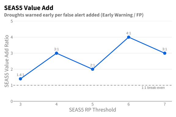
The key metric is FP (added) — false positives that SEAS5 contributes beyond what CDI already triggers. These are the alerts that actually hurt combined performance under OR logic.
RP ≥ 4 maximizes early warning value:
Raising to RP ≥ 5 drops recent droughts (2021, 2023) without benefit. Lowering to RP ≥ 3 adds more false alerts that CDI wouldn’t have triggered.
Our F1-tuned CDI threshold triggers 11 years, capturing 9 of 10 ASI-defined droughts. The 3 “problem years” reveal important limitations:
# Get probabilities from the fitted model
prob_drought <- predict(final_ridge_fit, df_apr, type = "prob")$.pred_yes

# Get ASI rankings from raw data
df_apr_ranked <- blob_read(name = FEATURE_PATHS$april, container = "projects") |>
    filter(!is.na(outcome_asi_zscore)) |>
    arrange(desc(outcome_asi_zscore)) |>
    mutate(asi_rank = row_number()) |>
    select(pub_year, outcome_asi_zscore, asi_rank)

df_analysis <- tibble(
    year = df_apr$pub_year,
    drought_actual = df_apr$drought,
    prob = prob_drought
) |>
    mutate(
        prob_rank = rank(-prob),
        triggered = prob > best_prob_threshold,
        status = case_when(
            triggered & drought_actual == "yes" ~ "TP",
            triggered & drought_actual == "no" ~ "FP",
            !triggered & drought_actual == "yes" ~ "FN",
            TRUE ~ "TN"
        )
    ) |>
left_join(df_apr_ranked, by = c("year" = "pub_year"))df_fp_fn <- df_analysis |>
filter(status %in% c("FP", "FN")) |>
arrange(status, desc(prob)) |>
select(year, status, prob, prob_rank, asi_rank, outcome_asi_zscore, drought_actual) |>
mutate(
prob = round(prob, 3),
outcome_asi_zscore = round(outcome_asi_zscore, 2)
)
df_fp_fn |>
rename(
Year = year,
Status = status,
`CDI Prob` = prob,
`Prob Rank` = prob_rank,
`ASI Rank` = asi_rank,
`ASI Z-score` = outcome_asi_zscore,
`ASI Drought` = drought_actual
) |>
gt() |>
tab_header(
title = "Model Errors: False Positives and False Negatives",
subtitle = "Comparing CDI probability rank vs ASI outcome rank"
) |>
tab_style(
style = cell_fill(color = "tomato", alpha = 0.3),
locations = cells_body(rows = df_fp_fn$status == "FP")
) |>
tab_style(
style = cell_fill(color = "steelblue", alpha = 0.3),
locations = cells_body(rows = df_fp_fn$status == "FN")
) |>
tab_footnote(
footnote = "FP = False Positive (triggered, not drought) | FN = False Negative (missed drought)",
locations = cells_column_labels(columns = Status)
)| Model Errors: False Positives and False Negatives | ||||||
| Comparing CDI probability rank vs ASI outcome rank | ||||||
| Year | Status1 | CDI Prob | Prob Rank | ASI Rank | ASI Z-score | ASI Drought |
|---|---|---|---|---|---|---|
| 2007 | FN | 0.053 | 32 | 5 | 1.30 | yes |
| 2004 | FP | 0.553 | 7 | 12 | 0.45 | no |
| 2000 | FP | 0.430 | 10 | 15 | 0.02 | no |
| 1 FP = False Positive (triggered, not drought) | FN = False Negative (missed drought) | ||||||
df_analysis |>
    ggplot(aes(x = asi_rank, y = prob_rank)) +
    geom_abline(slope = 1, intercept = 0, linetype = "dashed", color = "grey50") +
    geom_point(aes(color = status, size = status), alpha = 0.7) +
    geom_text(
        data = df_analysis |> filter(status %in% c("FP", "FN")),
        aes(label = year),
        hjust = -0.2, vjust = 0.5, size = 3
    ) +
    # Add reference lines for thresholds
    geom_hline(yintercept = 11.5, linetype = "dotted", color = hdx_hex("sapphire-hdx")) +
    geom_vline(xintercept = 10.5, linetype = "dotted", color = hdx_hex("tomato-hdx")) +
    annotate("text", x = 42, y = 11.5, label = "CDI threshold",
             hjust = 1, vjust = -0.5, size = 3, color = hdx_hex("sapphire-hdx")) +
    annotate("text", x = 10.5, y = 42, label = "ASI threshold",
             hjust = -0.1, vjust = 1, size = 3, color = hdx_hex("tomato-hdx"), angle = 90) +
    scale_color_manual(
        values = c("TP" = hdx_hex("mint-hdx"), "TN" = "grey70",
                   "FP" = hdx_hex("tomato-hdx"), "FN" = hdx_hex("sapphire-hdx")),
        labels = c("TP" = "True Positive", "TN" = "True Negative",
                   "FP" = "False Positive", "FN" = "False Negative")
    ) +
    scale_size_manual(values = c("TP" = 3, "TN" = 2, "FP" = 5, "FN" = 5), guide = "none") +
    scale_x_reverse() +
    scale_y_reverse() +
    labs(
        title = "CDI Probability Rank vs ASI Outcome Rank",
        subtitle = "Years in upper-left or lower-right quadrants are model errors",
        x = "ASI Rank (1 = worst drought)",
        y = "CDI Probability Rank (1 = highest prob)",
        color = NULL
    ) +
    theme(legend.position = "bottom")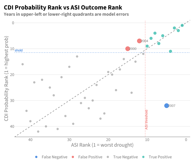
False Positives (2004, 2000): These years have indicator profiles that look like developing droughts in April, but the harvest-time ASI outcome was not severe. Possible explanations:
False Negative (2007): ASI ranks it as drought (rank 5), but CDI gives it very low probability. This is the “2007 Anomaly” discussed below — likely caused by fallow fields from 2006 drought displacement distorting the signal.
The scatterplot shows years on the diagonal are well-calibrated (ASI rank ≈ CDI rank). Off-diagonal years reveal where early indicators diverge from outcomes.
2007 consistently appears as a false positive across trigger configurations — the CDI triggers but the ASI outcome does not classify 2007 as a drought year. However, closer inspection suggests the outcome variable may be misleading, not the trigger.
The table below compares 2007’s indicator z-scores to the average across confirmed drought years:
cdi_component_cols <- cdi_weights$term

df_components_2007 <- df_apr |>
    mutate(year = pub_year) |>
    select(year, drought, all_of(cdi_component_cols))

# 2007 values
vals_2007 <- df_components_2007 |>
    filter(year == 2007) |>
    pivot_longer(cols = all_of(cdi_component_cols),
                 names_to = "component", values_to = "zscore_2007") |>
    select(component, zscore_2007)

# Drought year averages
vals_drought_avg <- df_components_2007 |>
    filter(drought == "yes") |>
    summarise(across(all_of(cdi_component_cols), mean)) |>
    pivot_longer(everything(), names_to = "component", values_to = "drought_avg")

# 2007 rank per component
vals_rank <- df_components_2007 |>
    mutate(across(
        all_of(cdi_component_cols),
        \(x) rank(-x, ties.method = "average"),
        .names = "{.col}_rank"
    )) |>
    filter(year == 2007) |>
    select(ends_with("_rank")) |>
    pivot_longer(everything(), names_to = "component", values_to = "rank") |>
    mutate(
        component = gsub("_rank$", "", component),
        component_rp = round(nrow(df_components_2007) / rank, 1)
    )

vals_2007 |>
    left_join(vals_drought_avg, by = "component") |>
    left_join(vals_rank, by = "component") |>
    select(component, zscore_2007, drought_avg, rank, component_rp) |>
    mutate(across(where(is.numeric), \(x) round(x, 2))) |>
    knitr::kable(
        col.names = c("Component", "2007 Z-score", "Drought Avg", "Rank (of 42)", "Component RP"),
        caption = "2007 component-level z-scores vs drought year averages"
)| Component | 2007 Z-score | Drought Avg | Rank (of 42) | Component RP |
|---|---|---|---|---|
| mixed_fcast_obsv | -0.82 | 0.82 | 35 | 1.2 |
| asi | -0.53 | 1.08 | 23 | 1.8 |
| snow_cover | -0.74 | 0.79 | 31 | 1.4 |
| vhi | 0.23 | 1.00 | 16 | 2.6 |
| volumetric_soil_water_1m | 0.02 | 1.01 | 23 | 1.8 |
2006 was a confirmed severe drought year. A Joint Appeal for Afghanistan Drought was launched in July 2006 due to inadequate April–May rainfall. UNHCR and ReliefWeb situation reports document significant displacement from exactly our AOI provinces (Faryab, Badghis, Sar-e-Pul, Balkh, Jawzjan) during the 2006 drought — families left, some dismantling their houses indicating no intent to return, and WFP planting surveys showed exceptionally low planting levels across Jawzjan, Faryab, and Samangan.
The likely mechanism for 2007’s anomalous ASI signal:
The 2007 case is instructive: the trigger system’s early-season indicators (precipitation forecasts, soil moisture, snow cover) correctly show no drought signal in 2007. The apparent false positive reflects a limitation of the outcome variable (ASI), not the trigger. If anything, a trigger system that does not fire for 2007 is behaving correctly — there was no meteorological drought to anticipate.
This means the true precision of the CDI trigger may be higher than the LOOCV estimate, since at least one “false positive” (2007) may actually be correct.
This section exports the final trigger thresholds as a single parquet file for use by the monitoring pipeline. It contains:
# --- SEAS5 RP6 z-score from empirical distribution ---
# Interpolate to find the exact z-score corresponding to RP=6
seas5_rp_to_z <- approxfun(
    x = df_historical$seas5_rp,
    y = df_historical$seas5_mam,
    rule = 2
)
seas5_zscore_rp6 <- seas5_rp_to_z(6)

# --- Load raw SEAS5 data to get mean/sd for back-transformation ---
# Replicates the feature set creation pipeline (data-raw/16_*)
PROVINCES_AOI <- c("Faryab", "Sar-e-Pul", "Jawzjan", "Balkh", "Badghis")

df_seas5_raw <- cumulus::pg_load_seas5_historical(
    iso3 = "AFG",
    adm_name = PROVINCES_AOI,
    adm_level = 1,
    convert_units = TRUE
)

# Area weights for province aggregation (same source as feature set creation)
df_area <- blob_read(
    name = "ds-aa-afg-drought/raw/vector/historical_era5_land_ndjfmam_lte2025.parquet",
    container = "projects"
) |>
    janitor::clean_names() |>
    filter(adm1_name %in% PROVINCES_AOI) |>
    distinct(adm1_name, shape_area)

# Aggregate to MAM season, March-issued forecasts, area-weighted regional mean
df_seas5_mam_mm <- cumulus::seas5_aggregate_forecast(
    df = df_seas5_raw,
    value = "mean",
    valid_months = c(3, 4, 5),
    by = c("iso3", "pcode", "name", "issued_date")
) |>
    filter(lubridate::month(issued_date) == 3) |>
    rename(adm1_name = name, value = mean) |>
    left_join(df_area, by = "adm1_name") |>
    group_by(issued_date) |>
    summarise(
        value = weighted.mean(value, w = shape_area, na.rm = TRUE),
        .groups = "drop"
    ) |>
    filter(lubridate::year(issued_date) >= 1984)

# Back-transform: z = -(value - mean) / sd  →  value = mean - z * sd
seas5_mean_mm <- mean(df_seas5_mam_mm$value)
seas5_sd_mm <- sd(df_seas5_mam_mm$value)
seas5_mm_rp6 <- seas5_mean_mm - seas5_zscore_rp6 * seas5_sd_mmdf_thresholds <- tibble(
indicator = c("seas5_mam", "cdi"),
window = c("march", "april"),
threshold_value = c(seas5_mm_rp6, cdi_threshold),
threshold_unit = c("mm", "cdi_index"),
rp_equivalent = c(6, rp_f1_equivalent),
w_mixed_fcast_obsv = c(NA_real_, cdi_weights$weight[cdi_weights$term == "mixed_fcast_obsv"]),
w_asi = c(NA_real_, cdi_weights$weight[cdi_weights$term == "asi"]),
w_snow_cover = c(NA_real_, cdi_weights$weight[cdi_weights$term == "snow_cover"]),
w_vhi = c(NA_real_, cdi_weights$weight[cdi_weights$term == "vhi"]),
w_volumetric_soil_water_1m = c(NA_real_, cdi_weights$weight[cdi_weights$term == "volumetric_soil_water_1m"])
)
df_thresholds |>
knitr::kable(
digits = 3,
caption = "Trigger thresholds for 2026 monitoring pipeline"
)| indicator | window | threshold_value | threshold_unit | rp_equivalent | w_mixed_fcast_obsv | w_asi | w_snow_cover | w_vhi | w_volumetric_soil_water_1m |
|---|---|---|---|---|---|---|---|---|---|
| seas5_mam | march | 129.828 | mm | 6.00 | NA | NA | NA | NA | NA |
| cdi | april | 0.503 | cdi_index | 3.91 | 0.275 | 0.206 | 0.205 | 0.192 | 0.121 |
# Sanity check: verify back-transformation by joining on year
df_verify <- df_seas5_mam_mm |>
    mutate(
        pub_year = lubridate::year(issued_date),
        derived_z = -(value - seas5_mean_mm) / seas5_sd_mm
    ) |>
    inner_join(
        tibble(pub_year = df_historical$year, feature_z = df_historical$seas5_mam),
        by = "pub_year"
    )

z_cor <- round(cor(df_verify$derived_z, df_verify$feature_z), 6)

cat(glue("**Back-transformation verification:**\n\n"))
Back-transformation verification:
cat(glue("- SEAS5 mean (mm): {round(seas5_mean_mm, 2)}\n\n"))cat(glue("- SEAS5 sd (mm): {round(seas5_sd_mm, 2)}\n\n"))cat(glue("- RP6 z-score: {round(seas5_zscore_rp6, 3)}\n\n"))cat(glue("- **RP6 threshold (mm): {round(seas5_mm_rp6, 2)}**\n\n"))cat(glue("- Correlation (re-derived z vs feature set z, joined by year): {z_cor}\n\n"))The z-scores and empirical RPs above use the full 1984–2025 SEAS5 record (42 years). Since ASI validation is only possible from 1991 onward, we check whether restricting the SEAS5 baseline to 1991–2024 (34 years) changes which years fire or shifts the mm threshold.
df_mm_all <- df_seas5_mam_mm |>
    mutate(year = lubridate::year(issued_date))

df_mm_1991 <- df_mm_all |>
    filter(year >= 1991, year <= 2024)

# Empirical RP under each baseline (low mm = drought = high RP)
df_mm_all <- df_mm_all |>
    mutate(rp_1984 = rp_empirical(value, direction = "1"))

df_mm_1991 <- df_mm_1991 |>
    mutate(rp_1991 = rp_empirical(value, direction = "1"))

# Join for comparison
df_rp_compare <- df_mm_all |>
    left_join(df_mm_1991 |> select(year, rp_1991), by = "year") |>
    arrange(value)

# Years firing at RP >= 6 under each baseline
years_fire_1984 <- df_rp_compare |> filter(rp_1984 >= 6) |> pull(year) |> sort()
years_fire_1991 <- df_rp_compare |> filter(!is.na(rp_1991), rp_1991 >= 6) |> pull(year) |> sort()

# Exact mm threshold: the maximum mm value among years with RP >= 6
# (i.e. the "wettest" year that still qualifies as RP6+ drought)
mm_exact_1984 <- max(df_rp_compare$value[df_rp_compare$rp_1984 >= 6])
mm_exact_1991 <- max(df_mm_1991$value[df_mm_1991$rp_1991 >= 6])

# 1991 baseline mean/sd for reference
seas5_mean_1991 <- mean(df_mm_1991$value)
seas5_sd_1991 <- sd(df_mm_1991$value)# Show all years with RP >= 6 under either baseline
df_fire_compare <- df_rp_compare |>
filter(rp_1984 >= 6 | (!is.na(rp_1991) & rp_1991 >= 6)) |>
mutate(
fires_1984 = if_else(rp_1984 >= 6, "yes", "no"),
fires_1991 = if_else(!is.na(rp_1991) & rp_1991 >= 6, "yes", "no")
) |>
arrange(value) |>
select(year, value, rp_1984, rp_1991, fires_1984, fires_1991) |>
mutate(across(c(value, rp_1984, rp_1991), \(x) round(x, 2)))
df_fire_compare |>
rename(
Year = year,
`MAM (mm)` = value,
`RP (1984)` = rp_1984,
`RP (1991)` = rp_1991,
`Fires (1984)` = fires_1984,
`Fires (1991)` = fires_1991
) |>
gt() |>
tab_header(
title = "SEAS5 RP ≥ 6: Baseline Comparison",
subtitle = glue("1984 baseline: {nrow(df_mm_all)} years | 1991 baseline: {nrow(df_mm_1991)} years")
) |>
tab_style(
style = cell_fill(color = "steelblue", alpha = 0.3),
locations = cells_body(columns = `Fires (1984)`, rows = df_fire_compare$fires_1984 == "yes")
) |>
tab_style(
style = cell_fill(color = "steelblue", alpha = 0.3),
locations = cells_body(columns = `Fires (1991)`, rows = df_fire_compare$fires_1991 == "yes")
)| SEAS5 RP ≥ 6: Baseline Comparison | |||||
| 1984 baseline: 43 years | 1991 baseline: 34 years | |||||
| Year | MAM (mm) | RP (1984) | RP (1991) | Fires (1984) | Fires (1991) |
|---|---|---|---|---|---|
| 2004 | 101.08 | 44.00 | 35.00 | yes | yes |
| 2001 | 104.69 | 22.00 | 17.50 | yes | yes |
| 2008 | 107.25 | 14.67 | 11.67 | yes | yes |
| 2000 | 118.26 | 11.00 | 8.75 | yes | yes |
| 1985 | 125.76 | 8.80 | NA | yes | no |
| 2018 | 126.23 | 7.33 | 7.00 | yes | yes |
| 2006 | 128.94 | 6.29 | 5.83 | yes | no |
same_years <- setequal(years_fire_1984, intersect(years_fire_1991, years_fire_1984))

cat("**MM threshold comparison:**\n\n")
MM threshold comparison:
cat(glue("| Baseline | N years | Mean (mm) | SD (mm) | Exact RP≥6 threshold (mm) |\n"))cat("|----------|---------|-----------|---------|---------------------------|\n")|———-|———|———–|———|—————————|
cat(glue("| 1984–2025 | {nrow(df_mm_all)} | {round(seas5_mean_mm, 2)} | {round(seas5_sd_mm, 2)} | {round(mm_exact_1984, 2)} |\n"))cat(glue("| 1991–2024 | {nrow(df_mm_1991)} | {round(seas5_mean_1991, 2)} | {round(seas5_sd_1991, 2)} | {round(mm_exact_1991, 2)} |\n"))cat(glue("| 1984 (interpolated) | {nrow(df_mm_all)} | — | — | {round(seas5_mm_rp6, 2)} |\n\n"))cat(glue("**Difference (exact):** {round(mm_exact_1991 - mm_exact_1984, 2)} mm\n\n"))Difference (exact): -2.72 mm
cat(glue("**Years firing (1984 baseline):** {paste(years_fire_1984, collapse = ', ')}\n\n"))Years firing (1984 baseline): 1985, 2000, 2001, 2004, 2006, 2008, 2018
cat(glue("**Years firing (1991 baseline):** {paste(years_fire_1991, collapse = ', ')}\n\n"))Years firing (1991 baseline): 2000, 2001, 2004, 2008, 2018
if (setequal(years_fire_1984[years_fire_1984 >= 1991], years_fire_1991)) {
    cat("The same years fire under both baselines (within the 1991–2024 overlap period).\n")
} else {
    only_1984 <- setdiff(years_fire_1984[years_fire_1984 >= 1991], years_fire_1991)
    only_1991 <- setdiff(years_fire_1991, years_fire_1984)
    if (length(only_1984) > 0) cat(glue("**Only fires under 1984 baseline:** {paste(only_1984, collapse = ', ')}\n\n"))
    if (length(only_1991) > 0) cat(glue("**Only fires under 1991 baseline:** {paste(only_1991, collapse = ', ')}\n\n"))
}
Only fires under 1984 baseline: 2006
df_seas5_ts <- df_seas5_mam_mm |>
    mutate(
        year = lubridate::year(issued_date),
        triggered = value <= seas5_mm_rp6,
        year_label = paste0("'", formatC(year %% 100, width = 2, flag = "0"))
    )

ggplot(df_seas5_ts, aes(x = year, y = value)) +
    geom_hline(
        yintercept = seas5_mm_rp6,
        linetype = "dashed", color = "grey40", linewidth = 0.6
    ) +
    annotate("text",
        x = max(df_seas5_ts$year), y = seas5_mm_rp6,
        label = glue("RP6 threshold: {round(seas5_mm_rp6, 1)} mm"),
        hjust = 1, vjust = -0.7, size = 3, color = "grey40"
    ) +
    geom_line(color = "grey70", linewidth = 0.4) +
    geom_point(aes(color = triggered), size = 2.5) +
    geom_text(
        data = \(d) filter(d, triggered),
        aes(label = year_label),
        vjust = -1, size = 2.8, color = hdx_hex("tomato-hdx")
    ) +
    scale_color_manual(
        values = c("FALSE" = hdx_hex("sapphire-hdx"), "TRUE" = hdx_hex("tomato-hdx")),
        labels = c("FALSE" = "No trigger", "TRUE" = "Triggered"),
        name = NULL
    ) +
    labs(
        title = "SEAS5 MAM Precipitation Forecast (March-issued)",
        subtitle = "Area-weighted regional mean | Triggered years fall below RP6 threshold",
        x = NULL,
        y = "MAM Precipitation (mm)"
    ) +
    theme(legend.position = "bottom")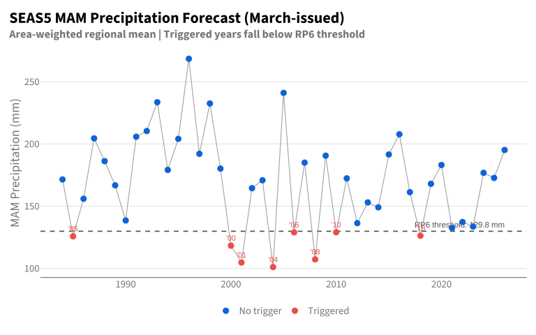
blob_write(
    df = df_thresholds,
    name = "ds-aa-afg-drought/monitoring_inputs/2026/trigger_thresholds.parquet",
    stage = "dev",
    container = "projects"
)The trigger thresholds have been written to blob at:
ds-aa-afg-drought/monitoring_inputs/2026/trigger_thresholds.parquet
To use in the monitoring pipeline:
threshold_value where indicator == "seas5_mam". Trigger if forecast ≤ threshold (low precipitation = drought).w_* columns, then compare against threshold_value where indicator == "cdi". Trigger if CDI ≥ threshold (high CDI = drought).Note: SEAS5 and CDI have opposite directionality — SEAS5 triggers on values below the threshold (dry forecast), CDI triggers on values above the threshold (drought signal).
Boolean activation history for both trigger windows. Uses the recommended configuration: SEAS5 RP ≥ 6 (Window 1, March) and CDI F1-optimized threshold (Window 2, April).
df_activation <- df_trigger |>
    transmute(
        year,
        afg_drought_v2_wt1 = seas5_rp6 == "yes",
        afg_drought_v2_wt2 = cdi_trig == "yes"
    ) |>
    arrange(year)

df_activation |>
    gt() |>
    tab_header(
        title = "Activation History: AFG Drought v2",
        subtitle = glue("{min(df_activation$year)}–{max(df_activation$year)} | wt1 = SEAS5 March, wt2 = CDI April")
    ) |>
    cols_label(
        year = "Year",
        afg_drought_v2_wt1 = "afg_drought_v2_wt1",
        afg_drought_v2_wt2 = "afg_drought_v2_wt2"
    ) |>
    tab_style(
        style = cell_fill(color = "tomato", alpha = 0.3),
        locations = cells_body(columns = afg_drought_v2_wt1, rows = df_activation$afg_drought_v2_wt1)
    ) |>
    tab_style(
        style = cell_fill(color = "tomato", alpha = 0.3),
        locations = cells_body(columns = afg_drought_v2_wt2, rows = df_activation$afg_drought_v2_wt2)
)| Activation History: AFG Drought v2 | ||
| 1984–2025 | wt1 = SEAS5 March, wt2 = CDI April | ||
| Year | afg_drought_v2_wt1 | afg_drought_v2_wt2 |
|---|---|---|
| 1984 | FALSE | FALSE |
| 1985 | TRUE | FALSE |
| 1986 | FALSE | FALSE |
| 1987 | FALSE | FALSE |
| 1988 | FALSE | FALSE |
| 1989 | FALSE | FALSE |
| 1990 | FALSE | FALSE |
| 1991 | FALSE | FALSE |
| 1992 | FALSE | FALSE |
| 1993 | FALSE | FALSE |
| 1994 | FALSE | FALSE |
| 1995 | FALSE | FALSE |
| 1996 | FALSE | FALSE |
| 1997 | FALSE | FALSE |
| 1998 | FALSE | FALSE |
| 1999 | FALSE | FALSE |
| 2000 | TRUE | TRUE |
| 2001 | TRUE | TRUE |
| 2002 | FALSE | FALSE |
| 2003 | FALSE | FALSE |
| 2004 | TRUE | TRUE |
| 2005 | FALSE | FALSE |
| 2006 | TRUE | TRUE |
| 2007 | FALSE | FALSE |
| 2008 | TRUE | TRUE |
| 2009 | FALSE | FALSE |
| 2010 | FALSE | FALSE |
| 2011 | FALSE | TRUE |
| 2012 | FALSE | FALSE |
| 2013 | FALSE | FALSE |
| 2014 | FALSE | FALSE |
| 2015 | FALSE | FALSE |
| 2016 | FALSE | FALSE |
| 2017 | FALSE | FALSE |
| 2018 | TRUE | TRUE |
| 2019 | FALSE | FALSE |
| 2020 | FALSE | FALSE |
| 2021 | FALSE | TRUE |
| 2022 | FALSE | TRUE |
| 2023 | FALSE | TRUE |
| 2024 | FALSE | FALSE |
| 2025 | FALSE | TRUE |
blob_write(
    df = df_activation,
    name = "ds-aa-cerf-global-trigger-allocations/aa_historical/yearly/v5/afg_drought_v2.csv",
    stage = "dev",
    container = "projects"
)