Appendix A — ASI Provincial Correlation Analysis

A.1 Intro

This chapter analyzes the correlation of end-of-season ASI (Agricultural Stress Index) values across Afghan provinces. We load dekadal ASI data from FAO at admin 1 level, filter to the end of season (May dekad 3), and examine both absolute values and Z-scores to understand how drought conditions co-vary spatially.

May dekad 3 represents the end of the spring wheat growing season, just as harvest begins, making it an appropriate time to measure cumulative drought stress.

Code
box::use(
    ../R/utils,
    dplyr[...],
    tidyr[...],
    lubridate[...],
    ggplot2[...],
    gghdx[...],
    corrplot[...],
    janitor[...],
    cumulus,
    purrr[...],
    stringr[...],
    tibble[deframe]
)
gghdx()

PROVINCES_AOI_WITH_BAMYAN <- c(
    "Faryab",
    "Sar-e-Pul",
    "Jawzjan",
    "Balkh",
    "Badghis",
    "Bamyan"
)

PROVINCES_AOI_NO_BAMYAN <- c(
    "Faryab",
    "Sar-e-Pul",
    "Jawzjan",
    "Balkh",
    "Badghis"
)

# Load CERF Rapid Response drought allocations for Afghanistan
df_cerf <- cumulus$blob_read(
    name = "ds-cerf-allocation-patterns/raw/CERF_allocation_by_year.csv",
    container = "projects",
    progress_show = FALSE
) |>
    filter(
        Country == "Afghanistan",
        str_detect(Emergency, regex("drought", ignore_case = TRUE)),
        Window == "Rapid Response"
    ) |>
    mutate(
        year = year(mdy(`Allocation date`))
    )

# Summarize by year for comparison plots
df_cerf_yearly <- df_cerf |>
    group_by(year) |>
    summarise(
        cerf_amount = sum(`Amount in US$`),
        cerf_n_allocations = n(),
        .groups = "drop"
    )

A.2 Helper Functions

Code
# Create correlation plot with consistent styling
plot_correlation_matrix <- function(cor_matrix, title) {
    corrplot(
        cor_matrix,
        method = "color",
        type = "lower",
        order = "hclust",
        tl.col = "black",
        tl.srt = 45,
        tl.cex = 0.9,
        addCoef.col = "black",
        number.cex = 0.7,
        title = title,
        mar = c(0, 0, 2, 0)
    )
}

# Calculate correlation matrix from wide data
calculate_correlation <- function(df_wide, exclude_cols = "year") {
    mat <- df_wide |>
        select(-all_of(exclude_cols)) |>
        as.matrix()

    cor(mat, use = "pairwise.complete.obs")
}

# Summarize correlation statistics
summarize_correlation <- function(cor_matrix) {
    lower_tri <- cor_matrix[lower.tri(cor_matrix)]

    tibble(
        mean = mean(lower_tri, na.rm = TRUE),
        min = min(lower_tri, na.rm = TRUE),
        max = max(lower_tri, na.rm = TRUE)
    )
}

# Perform hierarchical clustering and return results
perform_clustering <- function(df_wide,
                               province_col = "province",
                               dist_method = "euclidean",
                               hclust_method = "ward.D2") {
    mat <- df_wide |>
        select(-all_of(province_col)) |>
        as.matrix()

    rownames(mat) <- df_wide[[province_col]]

    dist_mat <- dist(mat, method = dist_method)
    hc <- hclust(dist_mat, method = hclust_method)

    list(
        matrix = mat,
        distance = dist_mat,
        hclust = hc
    )
}

# Plot dendrogram with optional cluster rectangles
plot_dendrogram <- function(hc, main_title, k = NULL, colors = NULL) {
    plot(
        hc,
        main = main_title,
        xlab = "Province",
        ylab = "Height",
        sub = ""
    )

    if (!is_null(k)) {
        rect.hclust(hc, k = k, border = colors)
    }
}

# Create cluster assignments for multiple k values
create_cluster_assignments <- function(hc, k_values) {
    cluster_list <- map(k_values, ~cutree(hc, k = .x))
    names(cluster_list) <- str_c("cluster_", k_values)

    tibble(province = names(cluster_list[[1]])) |>
        bind_cols(map_dfc(cluster_list, as.factor))
}

# Plot time series with cluster assignments
plot_timeseries_with_clusters <- function(df_asi, df_clusters,
                                         cluster_col = "cluster",
                                         title, subtitle) {
    n_clusters <- n_distinct(df_clusters[[cluster_col]])
    linetypes <- c("solid", "dashed", "dotted", "dotdash", "longdash")[1:n_clusters]

    df_asi |>
        left_join(df_clusters, by = "province") |>
        ggplot(aes(x = year, y = data, color = province, linetype = .data[[cluster_col]])) +
        geom_line(linewidth = 1) +
        geom_point(size = 2) +
        scale_linetype_manual(values = set_names(linetypes, as.character(1:n_clusters))) +
        labs(
            title = title,
            subtitle = subtitle,
            x = "Year",
            y = "ASI",
            color = "Province",
            linetype = "Cluster"
        ) +
        theme(legend.position = "bottom")
}

# Summarize clusters
summarize_clusters <- function(df_asi, df_clusters, cluster_col = "cluster") {
    df_asi |>
        left_join(df_clusters, by = "province") |>
        group_by(.data[[cluster_col]]) |>
        summarise(
            provinces = paste(unique(province), collapse = ", "),
            n_provinces = n_distinct(province),
            mean_asi = round(mean(data, na.rm = TRUE), 1),
            sd_asi = round(sd(data, na.rm = TRUE), 1),
            .groups = "drop"
        )
}

# Create threshold flags for multiple RP values
create_threshold_flags <- function(df_rp, rp_thresholds = c(3, 4, 5)) {
    for (rp in rp_thresholds) {
        flag_col <- str_c("flag_rp", rp)
        df_rp <- df_rp |>
            mutate({{flag_col}} := as.integer(rp >= !!rp))
    }
    df_rp
}

# Pivot threshold flags to wide format for all RP values
pivot_threshold_flags_wide <- function(df_flags, rp_thresholds = c(3, 4, 5)) {
    rp_thresholds |>
        map(~{
            flag_col <- str_c("flag_rp", .x)
            df_flags |>
                select(year, province, all_of(flag_col)) |>
                pivot_wider(names_from = province, values_from = all_of(flag_col)) |>
                arrange(year)
        }) |>
        set_names(str_c("rp", rp_thresholds))
}

# Plot threshold heatmap
plot_threshold_heatmap <- function(df_flags, title_suffix = "") {
    df_flags |>
        select(year, province, starts_with("flag_")) |>
        pivot_longer(
            cols = starts_with("flag"),
            names_to = "threshold",
            values_to = "exceeded"
        ) |>
        mutate(
            threshold = case_when(
                threshold == "flag_rp3" ~ "3-Year RP",
                threshold == "flag_rp4" ~ "4-Year RP",
                threshold == "flag_rp5" ~ "5-Year RP",
                TRUE ~ threshold
            ),
            threshold = factor(threshold, levels = c("3-Year RP", "4-Year RP", "5-Year RP"))
        ) |>
        ggplot(aes(x = year, y = province, fill = factor(exceeded))) +
        geom_tile(color = "white", linewidth = 0.5) +
    scale_x_continuous(breaks=1984:2025)+
        facet_wrap(~threshold, ncol = 1) +
        scale_fill_manual(
            values = c("0" = "gray90", "1" = "tomato"),
            labels = c("0" = "No", "1" = "Yes"),
            name = "Threshold\nExceeded"
        ) +
        labs(
            title = str_c("Return Period Threshold Exceedances", title_suffix),
            subtitle = "End-of-Season ASI (May Dekad 3)",
            x = "Year",
            y = "Province"
        ) +
        theme(
            axis.text.x = element_text(angle = 45, hjust = 1),
            panel.grid = element_blank()
        )
}

# Print correlation summary for multiple thresholds
print_correlation_summary <- function(cor_matrices, title_suffix = "") {
    cat(str_c("Correlation Summary by Threshold", title_suffix, ":\n\n"))

    walk2(cor_matrices, names(cor_matrices), ~{
        stats <- summarize_correlation(.x)
        threshold_name <- str_replace(.y, "rp", "") |>
            str_c("-Year RP Threshold")

        cat(threshold_name, ":\n", sep = "")
        cat("  Mean correlation:", round(stats$mean, 3), "\n")
        cat("  Range:", round(stats$min, 3), "to", round(stats$max, 3), "\n\n")
    })
}
A.3 Load ASI Data

Code
df_asi_raw <- cumulus::fao_asi_adm1_tabular(iso3 = "afg")

glimpse(df_asi_raw)
Rows: 40,031
Columns: 12
$ Indicator <chr> "Agricultural Stress Index (ASI)", "Agricultural Stress Inde…
$ Country   <chr> "Afghanistan", "Afghanistan", "Afghanistan", "Afghanistan", …
$ ADM1_CODE <dbl> 272, 272, 272, 272, 272, 272, 272, 272, 272, 272, 272, 272, …
$ Province  <chr> "Badakhshan", "Badakhshan", "Badakhshan", "Badakhshan", "Bad…
$ Land_Type <chr> "Crop Area", "Crop Area", "Crop Area", "Crop Area", "Crop Ar…
$ Date      <date> 1984-02-11, 1984-02-21, 1984-03-01, 1984-03-11, 1984-03-21,…
$ Data      <dbl> 0.000, 0.000, 1.676, 18.214, 20.486, 9.473, 6.116, 9.043, 6.…
$ Year      <dbl> 1984, 1984, 1984, 1984, 1984, 1984, 1984, 1984, 1984, 1984, …
$ Month     <chr> "02", "02", "03", "03", "03", "04", "04", "04", "05", "05", …
$ Dekad     <dbl> 2, 3, 1, 2, 3, 1, 2, 3, 1, 2, 3, 1, 2, 3, 1, 2, 3, 1, 2, 3, …
$ Unit      <chr> "% of area with Mean VHI below 35", "% of area with Mean VHI…
$ Source    <chr> "FAO-ASIS", "FAO-ASIS", "FAO-ASIS", "FAO-ASIS", "FAO-ASIS", …

A.4 Filter to End of Season (May Dekad 3)

The end of the spring wheat season in Afghanistan is May dekad 3 (approximately May 21-31). This is when ASI provides the most meaningful measure of cumulative drought impact on the season.

Code
df_asi_eos <- df_asi_raw |>
    clean_names() |>
    filter(
        month == "05",
        dekad == 3
    ) |>
    mutate(year = year(date))

# Check the data
df_asi_eos |>
    count(year) |>
    print(n = Inf)
# A tibble: 42 × 2
    year     n
   <dbl> <int>
 1  1984    34
 2  1985    34
 3  1986    34
 4  1987    34
 5  1988    34
 6  1989    34
 7  1990    34
 8  1991    34
 9  1992    34
10  1993    34
11  1994    34
12  1995    34
13  1996    34
14  1997    34
15  1998    34
16  1999    34
17  2000    34
18  2001    34
19  2002    34
20  2003    34
21  2004    34
22  2005    34
23  2006    34
24  2007    34
25  2008    34
26  2009    34
27  2010    34
28  2011    34
29  2012    34
30  2013    34
31  2014    34
32  2015    34
33  2016    34
34  2017    34
35  2018    34
36  2019    34
37  2020    34
38  2021    34
39  2022    34
40  2023    34
41  2024    34
42  2025    34
Code
# Pivot to wide format for correlation analysis
df_asi_wide <- df_asi_eos |>
    select(year, province, data) |>
    pivot_wider(
        names_from = province,
        values_from = data
    ) |>
    arrange(year)

df_asi_wide
# A tibble: 42 × 35
    year Badakhshan Badghis Baghlan  Balkh Bamyan Daykundi Farah Faryab Ghazni
   <dbl>      <dbl>   <dbl>   <dbl>  <dbl>  <dbl>    <dbl> <dbl>  <dbl>  <dbl>
 1  1984       1.82   0       0.041  0      0.275     0     0     0       0   
 2  1985      19.6   13.9     7.33   8.57  71.5      76.9  19.2   7.63   30.5 
 3  1986      52.0    0.342  75.9   70.2   60.8      23.8   1.28 16.7    39.2 
 4  1987      10.1    0.47    1.12   1.89  45.8       3.08  0     1.75    4.13
 5  1988       1.75   0.085   0.745  1.52   1.64      3.85  0     0.132   0   
 6  1989      88.7    2.82   32.8   14.0   97.8      69.2  73.1  40.4    61.1 
 7  1990      69.8    1.88   24.0   19.6   91.5      77.7  21.8  27.7    45.4 
 8  1991       9.21   0       0.911  2.35  64.4      39.2   1.28  0.132   7.28
 9  1992       3.17   0       0.124  1.72   0         0     0     0       0   
10  1993       1.26   0       0.58   0.761  0         0     0     0       0   
# ℹ 32 more rows
# ℹ 25 more variables: Ghor <dbl>, Hilmand <dbl>, Hirat <dbl>, Jawzjan <dbl>,
#   Kabul <dbl>, Kandahar <dbl>, Kapisa <dbl>, Khost <dbl>, Kunar <dbl>,
#   Kunduz <dbl>, Laghman <dbl>, Logar <dbl>, Nangarhar <dbl>, Nimroz <dbl>,
#   Nuristan <dbl>, Paktika <dbl>, Paktya <dbl>, Panjsher <dbl>, Parwan <dbl>,
#   Samangan <dbl>, `Sar-e-Pul` <dbl>, Takhar <dbl>, Uruzgan <dbl>,
#   Wardak <dbl>, Zabul <dbl>

A.5 Calculate Z-Scores per Province

Z-scores standardize each province’s ASI values relative to its own historical mean and standard deviation, allowing us to compare drought severity across provinces with different baseline conditions.

Code
df_asi_zscores <- df_asi_eos |>
    group_by(adm1_code, province) |>
    mutate(
        mean_asi = mean(data, na.rm = TRUE),
        sd_asi = sd(data, na.rm = TRUE),
        zscore = (data - mean_asi) / sd_asi
    ) |>
    ungroup()

# Summary statistics by province
df_asi_zscores |>
    group_by(province) |>
    summarise(
        n_years = n(),
        mean_asi = round(mean(data, na.rm = TRUE), 1),
        sd_asi = round(sd(data, na.rm = TRUE), 1),
        min_asi = round(min(data, na.rm = TRUE), 1),
        max_asi = round(max(data, na.rm = TRUE), 1),
        .groups = "drop"
    ) |>
    arrange(desc(mean_asi))
# A tibble: 34 × 6
   province n_years mean_asi sd_asi min_asi max_asi
   <chr>      <int>    <dbl>  <dbl>   <dbl>   <dbl>
 1 Nimroz        42     37.8   38.4       0   100  
 2 Ghazni        42     22.6   29.2       0    97  
 3 Hilmand       42     22.4   26.6       0    94.8
 4 Uruzgan       42     22     23         0    74.6
 5 Hirat         42     21.3   27.2       0    93.1
 6 Zabul         42     20.8   30.4       0    99.8
 7 Balkh         42     19.5   27.3       0    93.7
 8 Logar         42     19.3   23.7       0    98.7
 9 Ghor          42     19.2   29.7       0    90.6
10 Bamyan        42     18.8   27.5       0    97.8
# ℹ 24 more rows
Code
# Pivot Z-scores to wide format
df_zscore_wide <- df_asi_zscores |>
    select(year, province, zscore) |>
    pivot_wider(
        names_from = province,
        values_from = zscore
    ) |>
    arrange(year)

df_zscore_wide
# A tibble: 42 × 35
    year Badakhshan Badghis Baghlan    Balkh Bamyan Daykundi   Farah  Faryab
   <dbl>      <dbl>   <dbl>   <dbl>    <dbl>  <dbl>    <dbl>   <dbl>   <dbl>
 1  1984     -0.510 -0.558   -0.547 -0.715   -0.674   -0.671 -0.636  -0.648 
 2  1985      0.367 -0.0715  -0.267 -0.400    1.91     2.53   0.0219 -0.361 
 3  1986      1.96  -0.546    2.36   1.86     1.52     0.321 -0.592  -0.0207
 4  1987     -0.103 -0.542   -0.505 -0.645    0.977   -0.543 -0.636  -0.582 
 5  1988     -0.513 -0.555   -0.520 -0.659   -0.624   -0.511 -0.636  -0.643 
 6  1989      3.78  -0.460    0.709 -0.203    2.87     2.21   1.86    0.869 
 7  1990      2.85  -0.492    0.372  0.00486  2.64     2.56   0.110   0.392 
 8  1991     -0.145 -0.558   -0.513 -0.629    1.65     0.961 -0.592  -0.643 
 9  1992     -0.443 -0.558   -0.544 -0.652   -0.684   -0.671 -0.636  -0.648 
10  1993     -0.537 -0.558   -0.526 -0.687   -0.684   -0.671 -0.636  -0.648 
# ℹ 32 more rows
# ℹ 26 more variables: Ghazni <dbl>, Ghor <dbl>, Hilmand <dbl>, Hirat <dbl>,
#   Jawzjan <dbl>, Kabul <dbl>, Kandahar <dbl>, Kapisa <dbl>, Khost <dbl>,
#   Kunar <dbl>, Kunduz <dbl>, Laghman <dbl>, Logar <dbl>, Nangarhar <dbl>,
#   Nimroz <dbl>, Nuristan <dbl>, Paktika <dbl>, Paktya <dbl>, Panjsher <dbl>,
#   Parwan <dbl>, Samangan <dbl>, `Sar-e-Pul` <dbl>, Takhar <dbl>,
#   Uruzgan <dbl>, Wardak <dbl>, Zabul <dbl>

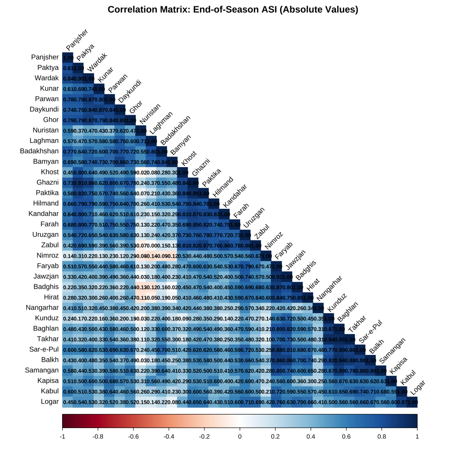
A.6 Correlation Matrix - Absolute ASI Values

This correlation matrix shows how end-of-season ASI values co-vary across provinces. High correlations indicate that provinces experience similar drought conditions in the same years.

Code
# Calculate and plot correlation matrix
cor_asi <- calculate_correlation(df_asi_wide)

plot_correlation_matrix(
    cor_asi,
    "Correlation Matrix: End-of-Season ASI (Absolute Values)"
)

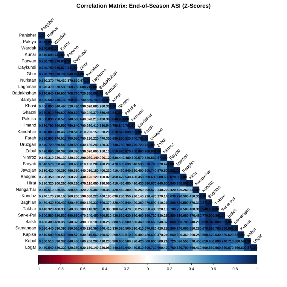
A.7 Correlation Matrix - Z-Scores

The Z-score correlation matrix examines whether standardized drought anomalies are correlated across provinces. This removes differences in baseline ASI levels and focuses on whether provinces experience above/below normal conditions together.

Code
# Calculate and plot correlation matrix
cor_zscore <- calculate_correlation(df_zscore_wide)

plot_correlation_matrix(
    cor_zscore,
    "Correlation Matrix: End-of-Season ASI (Z-Scores)"
)

A.8 Time Series Visualization

Code
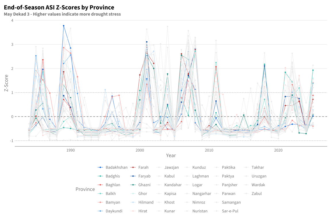
ggplot(
    df_asi_zscores,
    aes(x = year, y = zscore, color = province)
) +
    geom_line(alpha = 0.7) +
    geom_point(size = 1) +
    geom_hline(yintercept = 0, linetype = "dashed", color = "gray50") +
    geom_hline(yintercept = c(-1, 1), linetype = "dotted", color = "gray70") +
    labs(
        title = "End-of-Season ASI Z-Scores by Province",
        subtitle = "May Dekad 3 - Higher values indicate more drought stress",
        x = "Year",
        y = "Z-Score",
        color = "Province"
    ) +
    theme(legend.position = "bottom") +
    guides(color = guide_legend(ncol = 6))

A.9 Summary Statistics

Code
# Summary of correlations
cat("Absolute ASI Correlation Summary:\n")
Absolute ASI Correlation Summary:
Code
summarize_correlation(cor_asi) |>
    mutate(across(everything(), ~round(.x, 3))) |>
    print()
# A tibble: 1 × 3
   mean    min   max
  <dbl>  <dbl> <dbl>
1 0.512 -0.136 0.952
Code
cat("\nZ-Score Correlation Summary:\n")

Z-Score Correlation Summary:
Code
summarize_correlation(cor_zscore) |>
    mutate(across(everything(), ~round(.x, 3))) |>
    print()
# A tibble: 1 × 3
   mean    min   max
  <dbl>  <dbl> <dbl>
1 0.512 -0.136 0.952

A.10 Provincial Clustering Analysis

This section analyzes the provinces of interest using hierarchical clustering to group them based on their ASI patterns. We perform the analysis both with and without Bamyan to understand its influence.

Code
# Create a list of province sets to analyze
province_sets <- list(
    with_bamyan = PROVINCES_AOI_WITH_BAMYAN,
    without_bamyan = PROVINCES_AOI_NO_BAMYAN
)

# Filter and prepare data for each province set
df_asi_aoi_list <- map(province_sets, ~{
    df_asi_eos |>
        filter(province %in% .x)
})

# Create wide format matrices for clustering
df_asi_aoi_wide_list <- map(df_asi_aoi_list, ~{
    .x |>
        select(year, province, data) |>
        pivot_wider(
            names_from = year,
            values_from = data
        )
})

# Perform hierarchical clustering for each set
clustering_results <- map(df_asi_aoi_wide_list, ~{
    perform_clustering(.x, province_col = "province")
})

A.10.1 Clustering Analysis - AOI Provinces (Including Bamyan)

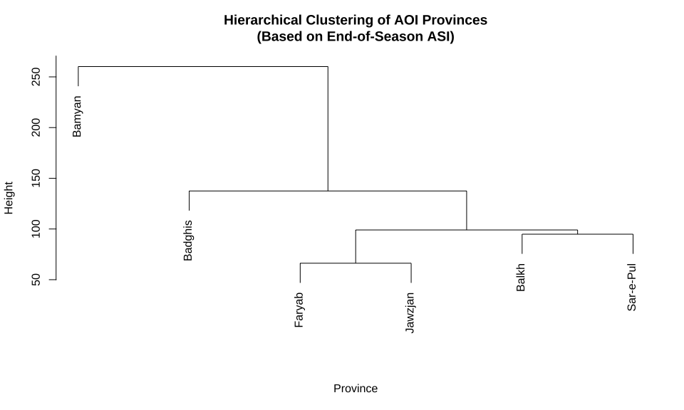
This section focuses on the provinces of interest (Northern: Faryab, Sar-e-Pul, Jawzjan, Balkh; Western: Badghis; Central: Bamyan) and uses hierarchical clustering to group them based on their ASI patterns.

Code
# Show the data matrix
clustering_results$with_bamyan$matrix
           1984   1985   1986   1987  1988   1989   1990   1991  1992  1993
Badghis   0.000 13.920  0.342  0.470 0.085  2.818  1.879  0.000 0.000 0.000
Balkh     0.000  8.573 70.209  1.887 1.523 13.969 19.629  2.350 1.721 0.761
Bamyan    0.275 71.507 60.822 45.753 1.644 97.808 91.507 64.384 0.000 0.000
Faryab    0.000  7.629 16.689  1.748 0.132 40.371 27.682  0.132 0.000 0.000
Jawzjan   0.000 26.055 45.688  7.156 5.138 25.138 11.009  0.000 0.000 0.000
Sar-e-Pul 0.000 18.926 36.772 13.384 0.227 44.302 49.531  3.723 0.000 0.000
          1994   1995   1996   1997  1998  1999   2000   2001  2002  2003
Badghis      0  0.384  0.128  0.000 0.000 0.000 46.968 99.744 0.000 0.000
Balkh        0  4.965  3.807  5.594 2.052 2.251  5.065 91.989 3.906 0.000
Bamyan       0 18.904 41.370 43.288 0.000 0.000  0.000 55.890 3.014 7.397
Faryab       0  0.106  1.192  0.000 0.000 0.000 10.596 99.947 0.000 0.000
Jawzjan      0  6.239  4.404  2.385 2.018 0.000  9.908 86.239 3.486 0.000
Sar-e-Pul    0  2.870  5.627  0.739 0.000 0.000  6.309 72.322 0.000 0.000
            2004 2005   2006   2007   2008 2009  2010   2011  2012  2013  2014
Badghis   28.992 0.00 38.429 17.378 97.353 0.00 0.085 20.410 1.110 0.128 0.769
Balkh     24.032 2.45 48.924 63.919 93.678 0.00 0.761 80.735 6.653 4.634 9.235
Bamyan     9.863 1.37 40.274 59.178 11.507 1.37 0.000  3.562 1.918 0.548 0.548
Faryab    30.861 0.00 33.272 62.649 92.371 0.00 0.450 34.490 1.139 0.000 2.464
Jawzjan   38.716 0.00  5.138 42.752 91.376 0.00 0.000 35.963 0.367 1.284 5.688
Sar-e-Pul 18.642 0.00 22.307 58.483 84.399 0.00 0.000 47.087 0.028 0.028 1.591
           2015  2016   2017   2018  2019  2020   2021   2022   2023   2024
Badghis   0.512 0.043 11.486 78.214 0.000 0.000 68.683 56.789 11.443  0.854
Balkh     4.634 9.302  9.103 39.077 4.397 3.365 14.869 41.887 52.003  7.451
Bamyan    0.000 0.000  0.822  4.658 2.192 6.027  2.740 14.521  8.219 10.685
Faryab    2.967 0.265  8.662 73.339 1.113 0.026 39.448 39.565 37.377  2.570
Jawzjan   0.000 1.284  0.367 83.610 1.468 0.183 14.453 41.187 49.355 13.028
Sar-e-Pul 0.767 0.057  2.756 21.944 0.172 0.171 27.453 48.212 17.988  0.485
            2025
Badghis   71.197
Balkh     57.494
Bamyan     7.945
Faryab    54.835
Jawzjan   47.417
Sar-e-Pul 20.148
Code
# Plot dendrogram
plot_dendrogram(
    clustering_results$with_bamyan$hclust,
    "Hierarchical Clustering of AOI Provinces\n(Based on End-of-Season ASI)"
)

Multi-Cluster Solutions (Including Bamyan)

Code
# Create cluster assignments for 2 and 3 clusters
df_clusters_with_bamyan <- create_cluster_assignments(
    clustering_results$with_bamyan$hclust,
    k_values = c(2, 3)
)

df_clusters_with_bamyan |>
    arrange(cluster_2, cluster_3, province)
# A tibble: 6 × 3
  province  cluster_2 cluster_3
  <chr>     <fct>     <fct>    
1 Badghis   1         1        
2 Balkh     1         2        
3 Faryab    1         2        
4 Jawzjan   1         2        
5 Sar-e-Pul 1         2        
6 Bamyan    2         3        
Code
# Plot dendrograms with cluster rectangles
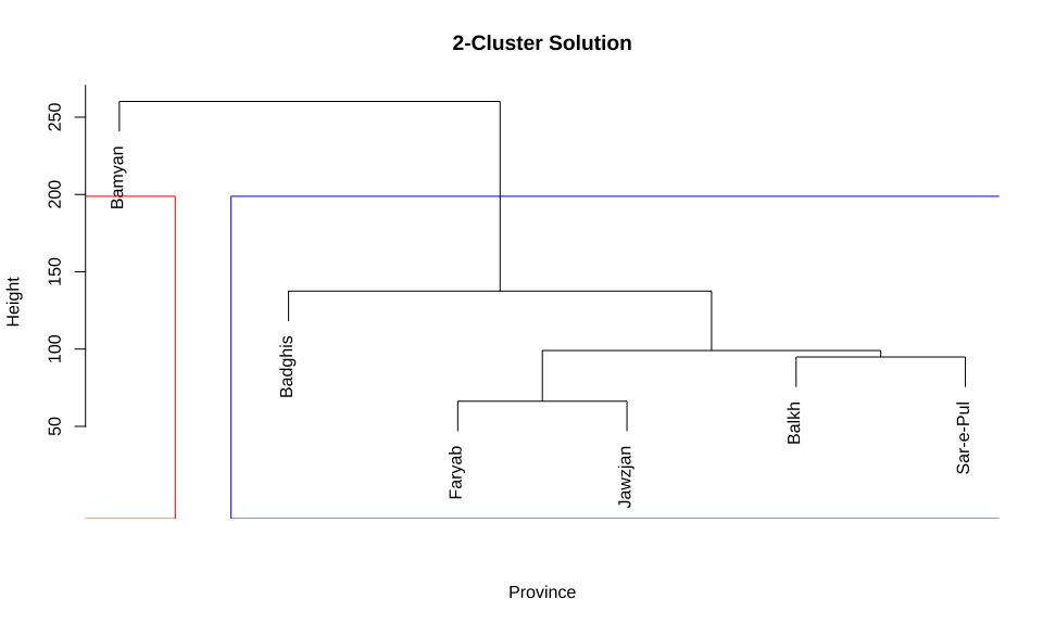
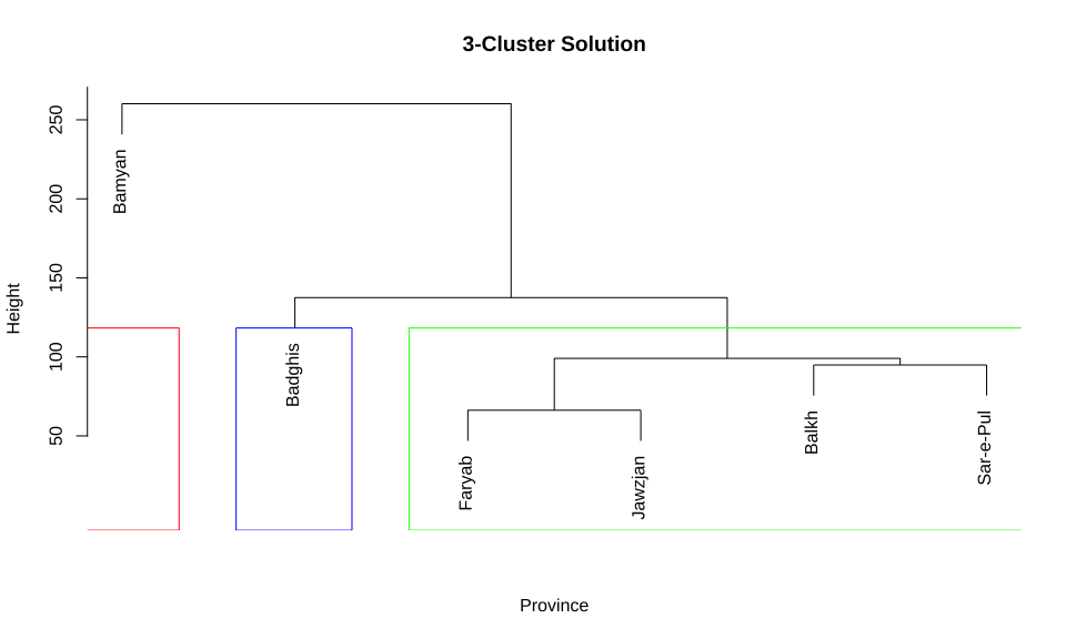
walk(c(2, 3), ~{
    plot_dendrogram(
        clustering_results$with_bamyan$hclust,
        str_c(.x, "-Cluster Solution"),
        k = .x,
        colors = c("red", "blue", "green")[1:.x]
    )
})

Code
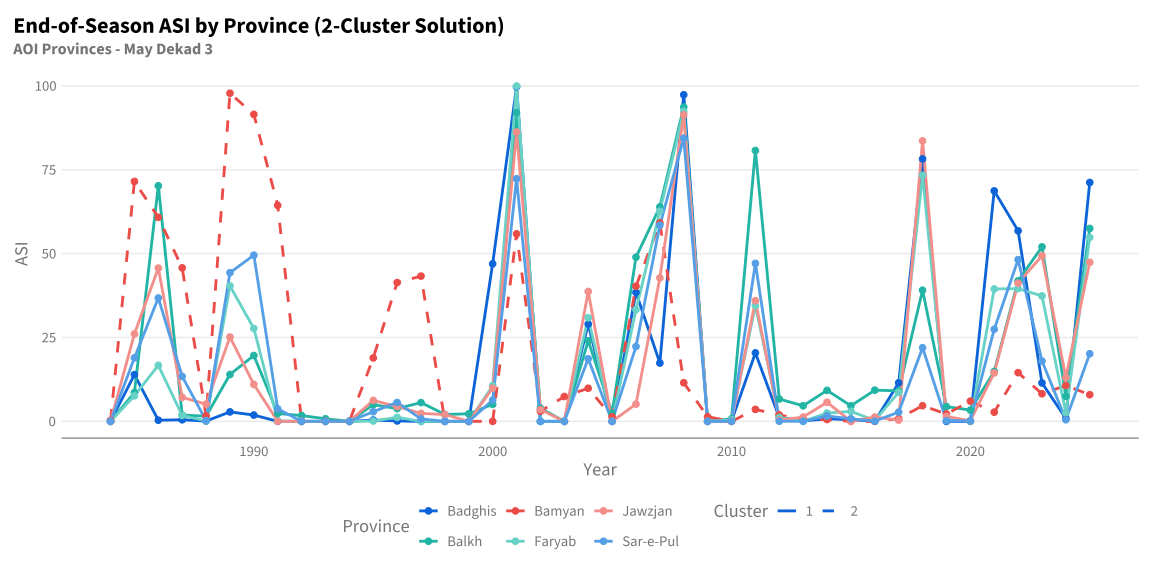
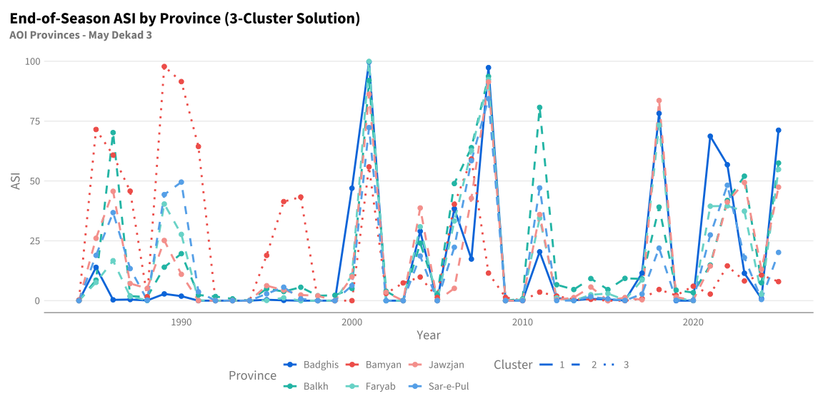
# Plot time series for each cluster solution
walk2(c(2, 3), c("cluster_2", "cluster_3"), ~{
    p <- plot_timeseries_with_clusters(
        df_asi_aoi_list$with_bamyan,
        df_clusters_with_bamyan |> select(province, cluster = all_of(.y)),
        cluster_col = "cluster",
        title = str_c("End-of-Season ASI by Province (", .x, "-Cluster Solution)"),
        subtitle = "AOI Provinces - May Dekad 3"
    )
    print(p)
})

Code
# Print cluster summaries
walk(c("cluster_2", "cluster_3"), ~{
    cat("\nSummary for", .x, ":\n")
    summarize_clusters(
        df_asi_aoi_list$with_bamyan,
        df_clusters_with_bamyan |> select(province, cluster = all_of(.x)),
        cluster_col = "cluster"
    ) |>
        print()
})

Summary for cluster_2 :
# A tibble: 2 × 5
  cluster provinces                                  n_provinces mean_asi sd_asi
  <fct>   <chr>                                            <int>    <dbl>  <dbl>
1 1       Badghis, Balkh, Faryab, Jawzjan, Sar-e-Pul           5     16.9   25.9
2 2       Bamyan                                               1     18.8   27.5

Summary for cluster_3 :
# A tibble: 3 × 5
  cluster provinces                         n_provinces mean_asi sd_asi
  <fct>   <chr>                                   <int>    <dbl>  <dbl>
1 1       Badghis                                     1     16     28.6
2 2       Balkh, Faryab, Jawzjan, Sar-e-Pul           4     17.1   25.2
3 3       Bamyan                                      1     18.8   27.5

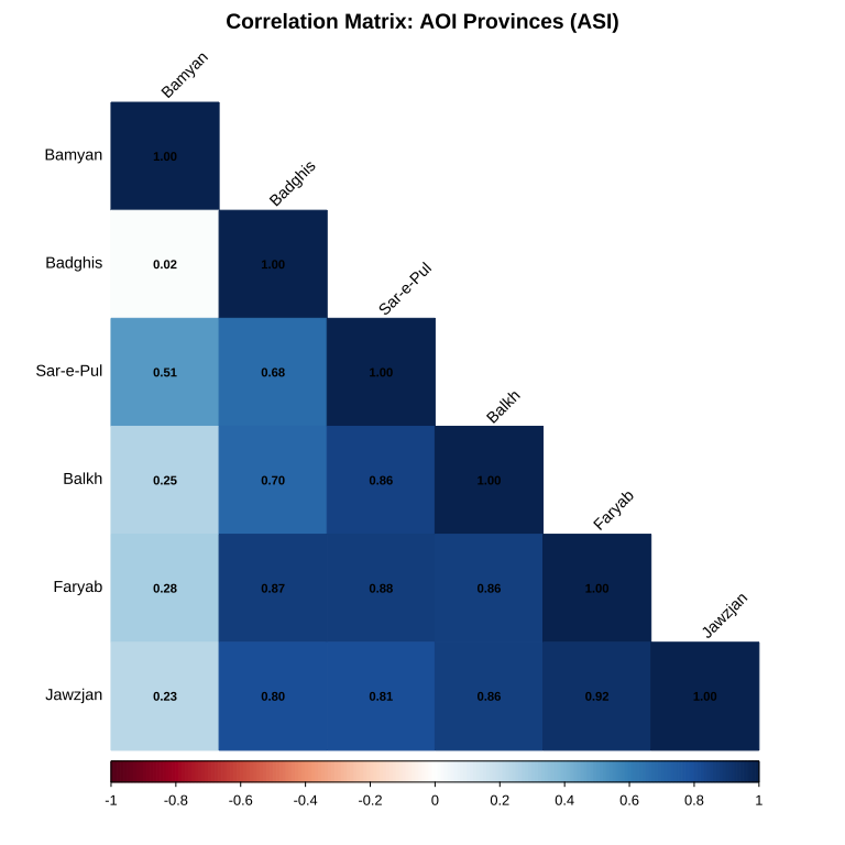
Cluster Correlation Heatmap (Including Bamyan)

Code
# Correlation matrix for AOI provinces
cor_aoi_with_bamyan <- cor(
    t(clustering_results$with_bamyan$matrix),
    use = "pairwise.complete.obs"
)

plot_correlation_matrix(
    cor_aoi_with_bamyan,
    "Correlation Matrix: AOI Provinces (ASI)"
)

A.10.2 Clustering Analysis - AOI Provinces (Excluding Bamyan)

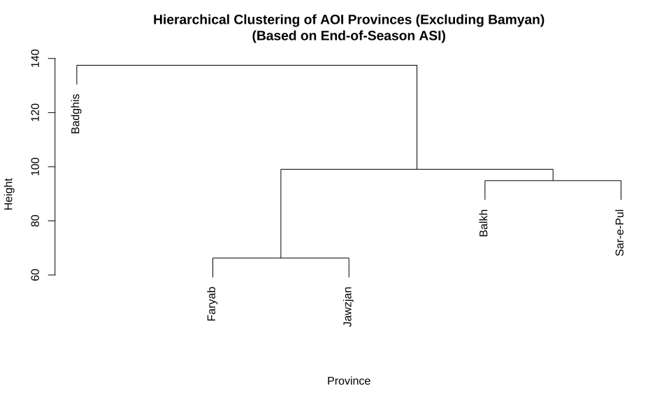
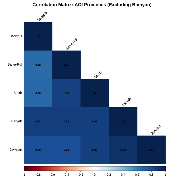
This section repeats the analysis excluding Bamyan (Central region), focusing only on Northern (Faryab, Sar-e-Pul, Jawzjan, Balkh) and Western (Badghis) provinces.

Code
# Show the data matrix
clustering_results$without_bamyan$matrix
          1984   1985   1986   1987  1988   1989   1990  1991  1992  1993 1994
Badghis      0 13.920  0.342  0.470 0.085  2.818  1.879 0.000 0.000 0.000    0
Balkh        0  8.573 70.209  1.887 1.523 13.969 19.629 2.350 1.721 0.761    0
Faryab       0  7.629 16.689  1.748 0.132 40.371 27.682 0.132 0.000 0.000    0
Jawzjan      0 26.055 45.688  7.156 5.138 25.138 11.009 0.000 0.000 0.000    0
Sar-e-Pul    0 18.926 36.772 13.384 0.227 44.302 49.531 3.723 0.000 0.000    0
           1995  1996  1997  1998  1999   2000   2001  2002 2003   2004 2005
Badghis   0.384 0.128 0.000 0.000 0.000 46.968 99.744 0.000    0 28.992 0.00
Balkh     4.965 3.807 5.594 2.052 2.251  5.065 91.989 3.906    0 24.032 2.45
Faryab    0.106 1.192 0.000 0.000 0.000 10.596 99.947 0.000    0 30.861 0.00
Jawzjan   6.239 4.404 2.385 2.018 0.000  9.908 86.239 3.486    0 38.716 0.00
Sar-e-Pul 2.870 5.627 0.739 0.000 0.000  6.309 72.322 0.000    0 18.642 0.00
            2006   2007   2008 2009  2010   2011  2012  2013  2014  2015  2016
Badghis   38.429 17.378 97.353    0 0.085 20.410 1.110 0.128 0.769 0.512 0.043
Balkh     48.924 63.919 93.678    0 0.761 80.735 6.653 4.634 9.235 4.634 9.302
Faryab    33.272 62.649 92.371    0 0.450 34.490 1.139 0.000 2.464 2.967 0.265
Jawzjan    5.138 42.752 91.376    0 0.000 35.963 0.367 1.284 5.688 0.000 1.284
Sar-e-Pul 22.307 58.483 84.399    0 0.000 47.087 0.028 0.028 1.591 0.767 0.057
            2017   2018  2019  2020   2021   2022   2023   2024   2025
Badghis   11.486 78.214 0.000 0.000 68.683 56.789 11.443  0.854 71.197
Balkh      9.103 39.077 4.397 3.365 14.869 41.887 52.003  7.451 57.494
Faryab     8.662 73.339 1.113 0.026 39.448 39.565 37.377  2.570 54.835
Jawzjan    0.367 83.610 1.468 0.183 14.453 41.187 49.355 13.028 47.417
Sar-e-Pul  2.756 21.944 0.172 0.171 27.453 48.212 17.988  0.485 20.148
Code
# Plot dendrogram
plot_dendrogram(
    clustering_results$without_bamyan$hclust,
    "Hierarchical Clustering of AOI Provinces (Excluding Bamyan)\n(Based on End-of-Season ASI)"
)

Multi-Cluster Solutions (Excluding Bamyan)

Code
# Create cluster assignments for 2 and 3 clusters
df_clusters_without_bamyan <- create_cluster_assignments(
    clustering_results$without_bamyan$hclust,
    k_values = c(2, 3)
)

df_clusters_without_bamyan |>
    arrange(cluster_2, cluster_3, province)
# A tibble: 5 × 3
  province  cluster_2 cluster_3
  <chr>     <fct>     <fct>    
1 Badghis   1         1        
2 Balkh     2         2        
3 Sar-e-Pul 2         2        
4 Faryab    2         3        
5 Jawzjan   2         3        
Code
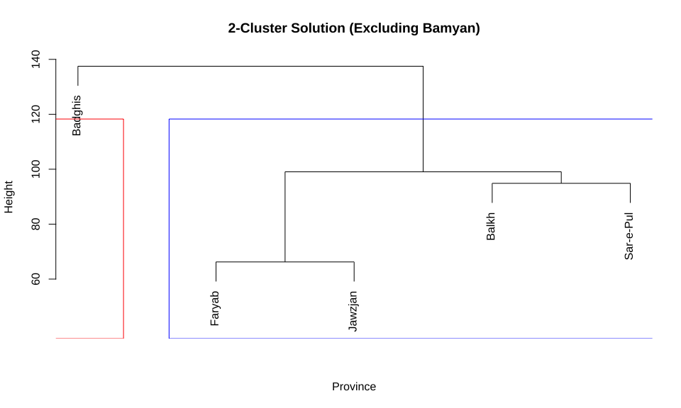
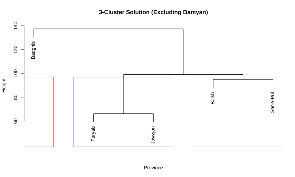
# Plot dendrograms with cluster rectangles
walk(c(2, 3), ~{
    plot_dendrogram(
        clustering_results$without_bamyan$hclust,
        str_c(.x, "-Cluster Solution (Excluding Bamyan)"),
        k = .x,
        colors = c("red", "blue", "green")[1:.x]
    )
})

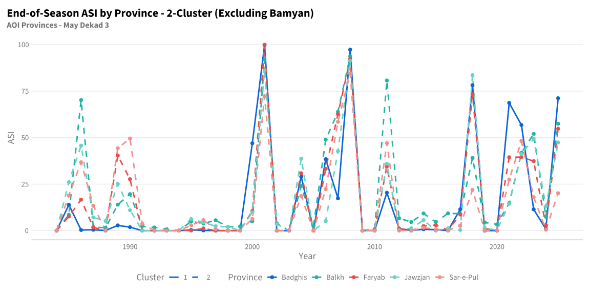
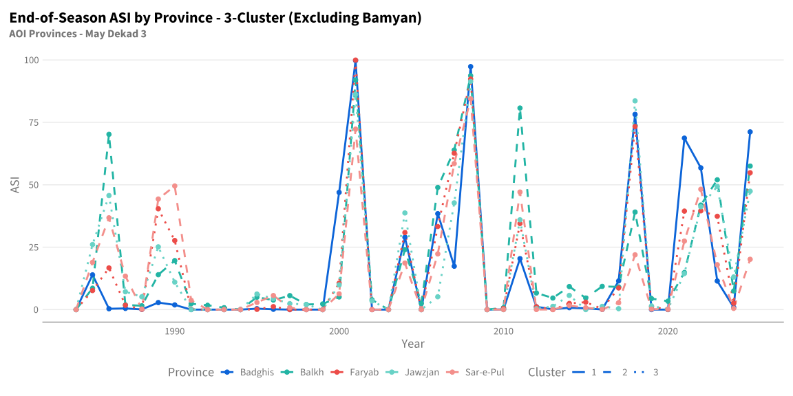
Code
# Plot time series for each cluster solution
walk2(c(2, 3), c("cluster_2", "cluster_3"), ~{
    p <- plot_timeseries_with_clusters(
        df_asi_aoi_list$without_bamyan,
        df_clusters_without_bamyan |> select(province, cluster = all_of(.y)),
        cluster_col = "cluster",
        title = str_c("End-of-Season ASI by Province - ", .x, "-Cluster (Excluding Bamyan)"),
        subtitle = "AOI Provinces - May Dekad 3"
    )
    print(p)
})

Code
# Print cluster summaries
walk(c("cluster_2", "cluster_3"), ~{
    cat("\nSummary for", .x, "(excluding Bamyan):\n")
    summarize_clusters(
        df_asi_aoi_list$without_bamyan,
        df_clusters_without_bamyan |> select(province, cluster = all_of(.x)),
        cluster_col = "cluster"
    ) |>
        print()
})

Summary for cluster_2 (excluding Bamyan):
# A tibble: 2 × 5
  cluster provinces                         n_provinces mean_asi sd_asi
  <fct>   <chr>                                   <int>    <dbl>  <dbl>
1 1       Badghis                                     1     16     28.6
2 2       Balkh, Faryab, Jawzjan, Sar-e-Pul           4     17.1   25.2

Summary for cluster_3 (excluding Bamyan):
# A tibble: 3 × 5
  cluster provinces        n_provinces mean_asi sd_asi
  <fct>   <chr>                  <int>    <dbl>  <dbl>
1 1       Badghis                    1     16     28.6
2 2       Balkh, Sar-e-Pul           2     17.2   24.8
3 3       Faryab, Jawzjan            2     17.1   25.8

Correlation Heatmap (Excluding Bamyan)

Code
# Correlation matrix for AOI provinces
cor_aoi_without_bamyan <- cor(
    t(clustering_results$without_bamyan$matrix),
    use = "pairwise.complete.obs"
)

plot_correlation_matrix(
    cor_aoi_without_bamyan,
    "Correlation Matrix: AOI Provinces (Excluding Bamyan)"
)

A.11 Return Period Threshold Analysis

This section calculates empirical return periods for end-of-season ASI by province and examines correlations based on threshold exceedance. Higher ASI values indicate more drought stress, so we use direction = "-1" (higher values = rarer events = higher RP).

We perform this analysis for both province sets (with and without Bamyan).

Code
# Calculate return periods for both province sets
df_asi_rp_list <- map(df_asi_aoi_list, ~{
    .x |>
        group_by(province) |>
        mutate(
            rp = utils$rp_empirical(x = data, direction = "-1", ties_method = "average")
        ) |>
        ungroup()
})

# View return periods for provinces with Bamyan
df_asi_rp_list$with_bamyan |>
    select(year, province, data, rp) |>
    arrange(province, desc(rp)) |>
    print(n = 30)
# A tibble: 252 × 4
    year province   data    rp
   <dbl> <chr>     <dbl> <dbl>
 1  2001 Badghis  99.7   43   
 2  2008 Badghis  97.4   21.5 
 3  2018 Badghis  78.2   14.3 
 4  2025 Badghis  71.2   10.8 
 5  2021 Badghis  68.7    8.6 
 6  2022 Badghis  56.8    7.17
 7  2000 Badghis  47.0    6.14
 8  2006 Badghis  38.4    5.38
 9  2004 Badghis  29.0    4.78
10  2011 Badghis  20.4    4.3 
11  2007 Badghis  17.4    3.91
12  1985 Badghis  13.9    3.58
13  2017 Badghis  11.5    3.31
14  2023 Badghis  11.4    3.07
15  1989 Badghis   2.82   2.87
16  1990 Badghis   1.88   2.69
17  2012 Badghis   1.11   2.53
18  2024 Badghis   0.854  2.39
19  2014 Badghis   0.769  2.26
20  2015 Badghis   0.512  2.15
21  1987 Badghis   0.47   2.05
22  1995 Badghis   0.384  1.95
23  1986 Badghis   0.342  1.87
24  1996 Badghis   0.128  1.76
25  2013 Badghis   0.128  1.76
26  1988 Badghis   0.085  1.62
27  2010 Badghis   0.085  1.62
28  2016 Badghis   0.043  1.54
29  1984 Badghis   0      1.21
30  1991 Badghis   0      1.21
# ℹ 222 more rows

A.11.1 Binary Threshold Flags

Create binary indicators for whether each province-year exceeds 3-year, 4-year, and 5-year return period thresholds.

Code
# Create threshold flags for both sets
df_asi_flags_list <- map(df_asi_rp_list, ~{
    create_threshold_flags(.x, rp_thresholds = c(3, 4, 5))
})

# Summary of threshold exceedances by province (with Bamyan)
df_asi_flags_list$with_bamyan |>
    group_by(province) |>
    summarise(
        n_years = n(),
        n_rp3 = sum(flag_rp3),
        n_rp4 = sum(flag_rp4),
        n_rp5 = sum(flag_rp5),
        pct_rp3 = round(100 * mean(flag_rp3), 1),
        pct_rp4 = round(100 * mean(flag_rp4), 1),
        pct_rp5 = round(100 * mean(flag_rp5), 1),
        .groups = "drop"
    ) |>
    arrange(province)
# A tibble: 6 × 8
  province  n_years n_rp3 n_rp4 n_rp5 pct_rp3 pct_rp4 pct_rp5
  <chr>       <int> <int> <int> <int>   <dbl>   <dbl>   <dbl>
1 Badghis        42    14    10     8    33.3    23.8      19
2 Balkh          42    14    10     8    33.3    23.8      19
3 Bamyan         42    14    10     8    33.3    23.8      19
4 Faryab         42    14    10     8    33.3    23.8      19
5 Jawzjan        42    14    10     8    33.3    23.8      19
6 Sar-e-Pul      42    14    10     8    33.3    23.8      19
Code
# Show which years exceeded each threshold by province
df_asi_flags_list$with_bamyan |>
    filter(flag_rp3 == 1) |>
    select(year, province, data, rp, flag_rp3, flag_rp4, flag_rp5) |>
    arrange(year, province)
# A tibble: 84 × 7
    year province   data    rp flag_rp3 flag_rp4 flag_rp5
   <dbl> <chr>     <dbl> <dbl>    <int>    <int>    <int>
 1  1985 Badghis    13.9  3.58        1        0        0
 2  1985 Bamyan     71.5 14.3         1        1        1
 3  1985 Jawzjan    26.1  3.91        1        0        0
 4  1985 Sar-e-Pul  18.9  3.31        1        0        0
 5  1986 Balkh      70.2 10.8         1        1        1
 6  1986 Bamyan     60.8  8.6         1        1        1
 7  1986 Faryab     16.7  3.07        1        0        0
 8  1986 Jawzjan    45.7  7.17        1        1        1
 9  1986 Sar-e-Pul  36.8  5.38        1        1        1
10  1987 Bamyan     45.8  5.38        1        1        1
# ℹ 74 more rows

A.12 Review of 2025

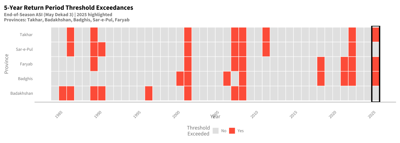
This section provides a quick visual summary of 2025 ASI threshold exceedances in context of the historical record for the provinces monitored in 2025.

Code
# Get provinces used in 2025 monitoring
provinces_2025 <- utils$load_aoi_names()

# Calculate RP and threshold flags for 2025 monitoring provinces
df_asi_2025_review <- df_asi_eos |>
    filter(province %in% provinces_2025) |>
    group_by(province) |>
    mutate(
        rp = utils$rp_empirical(x = data, direction = "-1", ties_method = "average"),
        flag_rp5 = as.integer(rp >= 5)
    ) |>
    ungroup()

# Plot RP=5 threshold exceedances with 2025 highlighted
df_asi_2025_review |>
    select(year, province, flag_rp5) |>
    mutate(exceeded = factor(flag_rp5, levels = c(0, 1))) |>
    ggplot(aes(x = year, y = province, fill = exceeded)) +
    geom_tile(color = "white", linewidth = 0.5) +
    annotate(
        "rect",
        xmin = 2024.5, xmax = 2025.5,
        ymin = -Inf, ymax = Inf,
        fill = NA, color = "black", linewidth = 1.5
    ) +
    scale_x_continuous(breaks = seq(1985, 2025, by = 5)) +
    scale_fill_manual(
        values = c("0" = "gray90", "1" = "tomato"),
        labels = c("0" = "No", "1" = "Yes"),
        name = "Threshold\nExceeded"
    ) +
    labs(
        title = "5-Year Return Period Threshold Exceedances",
        subtitle = str_c("End-of-Season ASI (May Dekad 3) | 2025 highlighted\nProvinces: ", paste(provinces_2025, collapse = ", ")),
        x = "Year",
        y = "Province"
    ) +
    theme(
        axis.text.x = element_text(angle = 45, hjust = 1),
        panel.grid = element_blank()
    )

A.12.1 Correlation by Threshold Exceedance

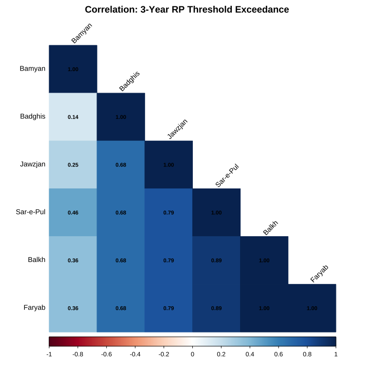
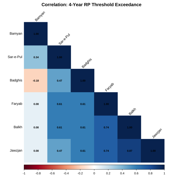
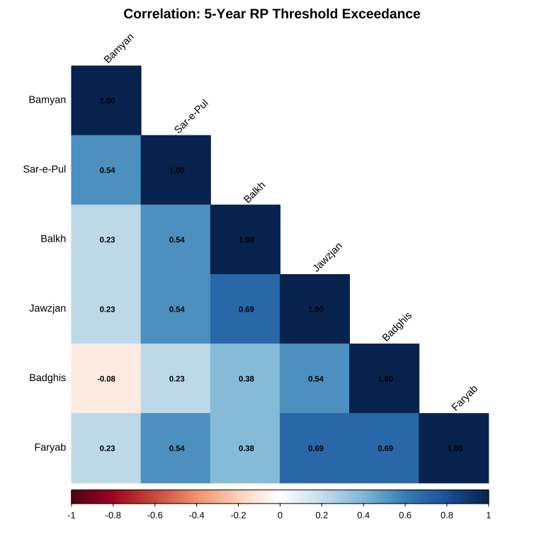
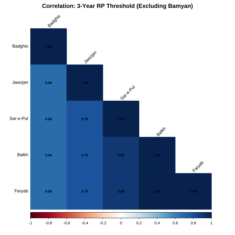
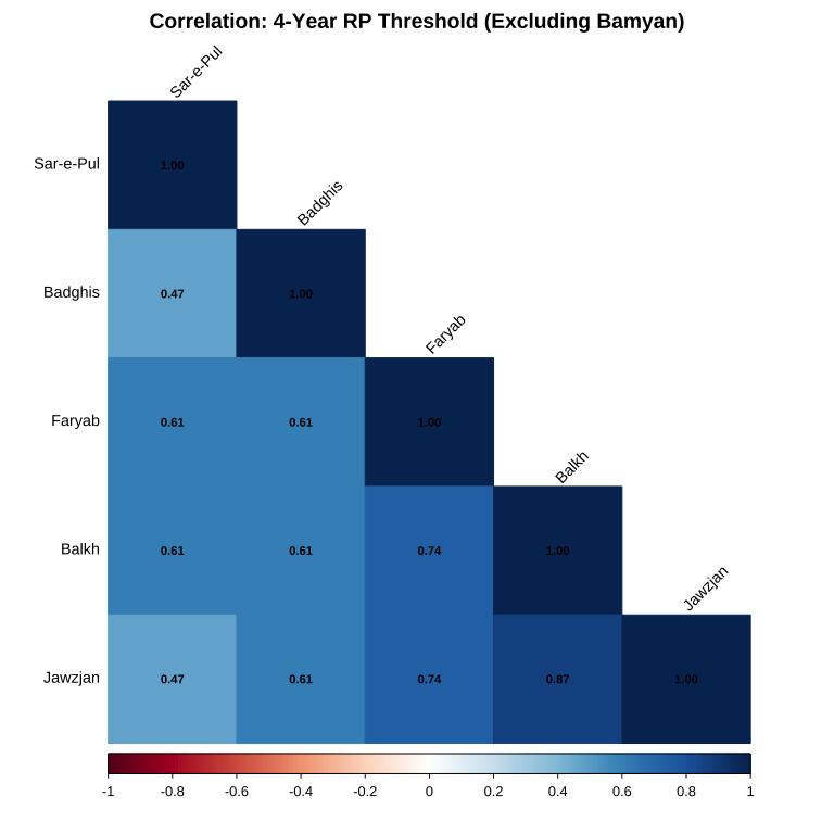
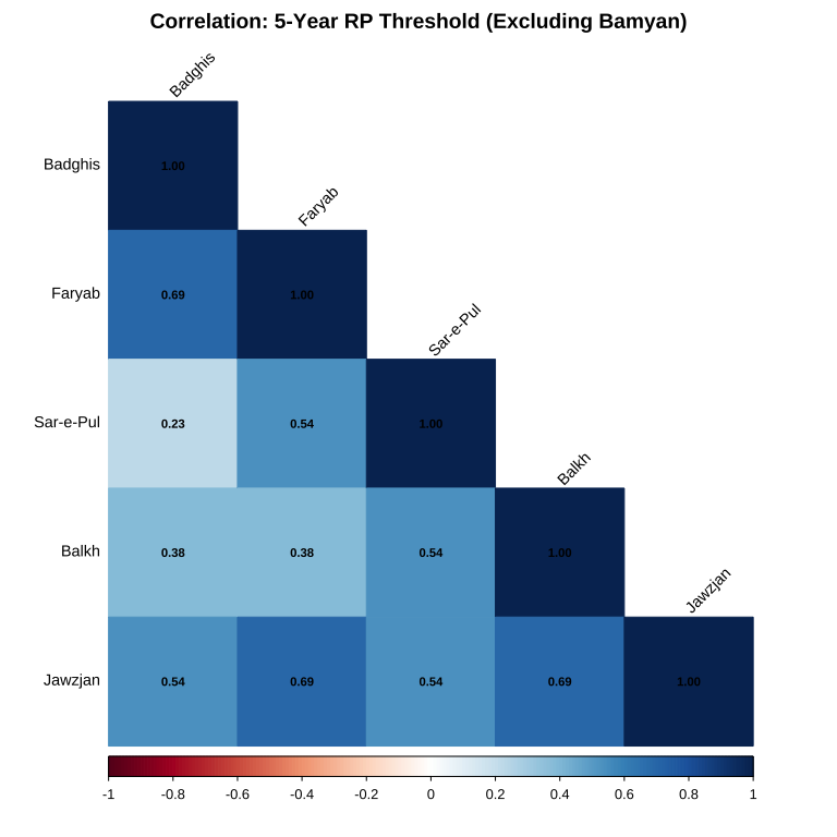
Calculate correlations between provinces based on whether they exceed thresholds in the same years. High correlation means provinces tend to experience severe drought (threshold exceedance) together.

Code
# Pivot threshold flags to wide format for both sets
df_flag_wide_list <- map(df_asi_flags_list, ~{
    pivot_threshold_flags_wide(.x, rp_thresholds = c(3, 4, 5))
})

With Bamyan - Threshold Correlations

Code
# Calculate correlations for each threshold
cor_rp_with_bamyan <- map(df_flag_wide_list$with_bamyan, ~{
    calculate_correlation(.x, exclude_cols = "year")
})

# Plot correlation matrices for each threshold
walk2(
    cor_rp_with_bamyan,
    c("3-Year", "4-Year", "5-Year"),
    ~plot_correlation_matrix(.x, str_c("Correlation: ", .y, " RP Threshold Exceedance"))
)

Without Bamyan - Threshold Correlations

Code
# Calculate correlations for each threshold
cor_rp_without_bamyan <- map(df_flag_wide_list$without_bamyan, ~{
    calculate_correlation(.x, exclude_cols = "year")
})

# Plot correlation matrices for each threshold
walk2(
    cor_rp_without_bamyan,
    c("3-Year", "4-Year", "5-Year"),
    ~plot_correlation_matrix(.x, str_c("Correlation: ", .y, " RP Threshold (Excluding Bamyan)"))
)

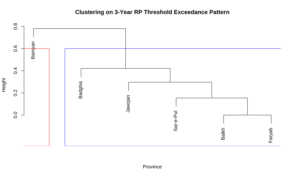
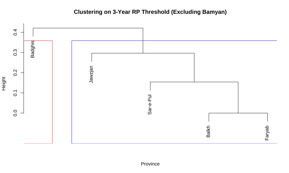
A.12.2 Clustering on Threshold Exceedance

Cluster provinces based on their pattern of threshold exceedances across all years.

Code
# Prepare matrices and perform clustering for 3-year RP threshold
clustering_rp3_results <- map(df_asi_flags_list, ~{
    df_wide <- .x |>
        select(year, province, flag_rp3) |>
        pivot_wider(names_from = year, values_from = flag_rp3)

    perform_clustering(df_wide, province_col = "province", dist_method = "binary")
})

Clustering - With Bamyan

Code
plot_dendrogram(
    clustering_rp3_results$with_bamyan$hclust,
    "Clustering on 3-Year RP Threshold Exceedance Pattern",
    k = 2,
    colors = c("red", "blue")
)

Code
# Create cluster assignments
df_clusters_rp3_with_bamyan <- create_cluster_assignments(
    clustering_rp3_results$with_bamyan$hclust,
    k_values = c(2, 3)
)

df_clusters_rp3_with_bamyan |>
    arrange(cluster_2, cluster_3, province)
# A tibble: 6 × 3
  province  cluster_2 cluster_3
  <chr>     <fct>     <fct>    
1 Badghis   1         1        
2 Balkh     1         2        
3 Faryab    1         2        
4 Jawzjan   1         2        
5 Sar-e-Pul 1         2        
6 Bamyan    2         3        

Clustering - Without Bamyan

Code
plot_dendrogram(
    clustering_rp3_results$without_bamyan$hclust,
    "Clustering on 3-Year RP Threshold (Excluding Bamyan)",
    k = 2,
    colors = c("red", "blue")
)

Code
# Create cluster assignments
df_clusters_rp3_without_bamyan <- create_cluster_assignments(
    clustering_rp3_results$without_bamyan$hclust,
    k_values = c(2, 3)
)

df_clusters_rp3_without_bamyan |>
    arrange(cluster_2, cluster_3, province)
# A tibble: 5 × 3
  province  cluster_2 cluster_3
  <chr>     <fct>     <fct>    
1 Badghis   1         1        
2 Balkh     2         2        
3 Faryab    2         2        
4 Sar-e-Pul 2         2        
5 Jawzjan   2         3        

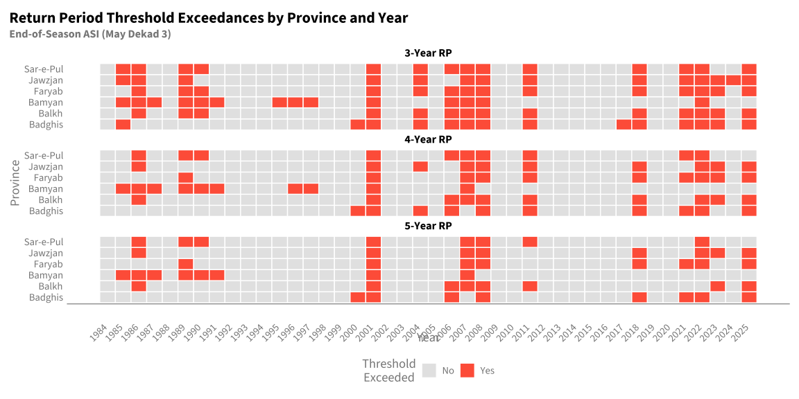
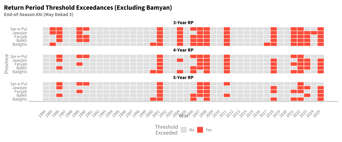
A.12.3 Threshold Exceedance Heatmaps

Code
# Visualize threshold exceedances as heatmap
plot_threshold_heatmap(
    df_asi_flags_list$with_bamyan,
    title_suffix = " by Province and Year"
)

Code
# Visualize threshold exceedances as heatmap (excluding Bamyan)
plot_threshold_heatmap(
    df_asi_flags_list$without_bamyan,
    title_suffix = " (Excluding Bamyan)"
)

A.12.4 Comparison: ASI Clustering vs Threshold Clustering

Code
# Compare clustering results for provinces with Bamyan
df_compare_clusters <- df_clusters_with_bamyan |>
    select(province, cluster_asi = cluster_2) |>
    left_join(
        df_clusters_rp3_with_bamyan |> select(province, cluster_rp3 = cluster_2),
        by = "province"
    )

df_compare_clusters |>
    arrange(cluster_asi, cluster_rp3)
# A tibble: 6 × 3
  province  cluster_asi cluster_rp3
  <chr>     <fct>       <fct>      
1 Badghis   1           1          
2 Balkh     1           1          
3 Faryab    1           1          
4 Jawzjan   1           1          
5 Sar-e-Pul 1           1          
6 Bamyan    2           2          

A.12.5 Correlation Summaries by Threshold

Code
# Print correlation summaries for provinces with Bamyan
print_correlation_summary(cor_rp_with_bamyan)
Correlation Summary by Threshold:

3-Year RP Threshold:
  Mean correlation: 0.629 
  Range: 0.143 to 1 

4-Year RP Threshold:
  Mean correlation: 0.449 
  Range: -0.181 to 0.869 

5-Year RP Threshold:
  Mean correlation: 0.424 
  Range: -0.081 to 0.691 
Code
cat("\n")
Code
# Print correlation summaries for provinces without Bamyan
print_correlation_summary(cor_rp_without_bamyan, title_suffix = " (Excluding Bamyan)")
Correlation Summary by Threshold (Excluding Bamyan):

3-Year RP Threshold:
  Mean correlation: 0.786 
  Range: 0.679 to 1 

4-Year RP Threshold:
  Mean correlation: 0.632 
  Range: 0.475 to 0.869 

5-Year RP Threshold:
  Mean correlation: 0.521 
  Range: 0.228 to 0.691 

A.13 Combined Return Period Analysis

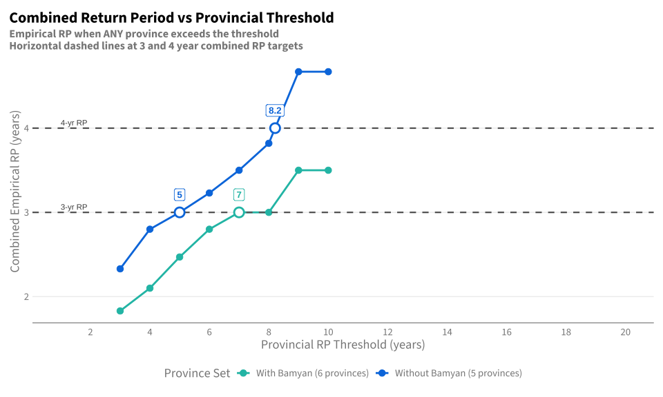
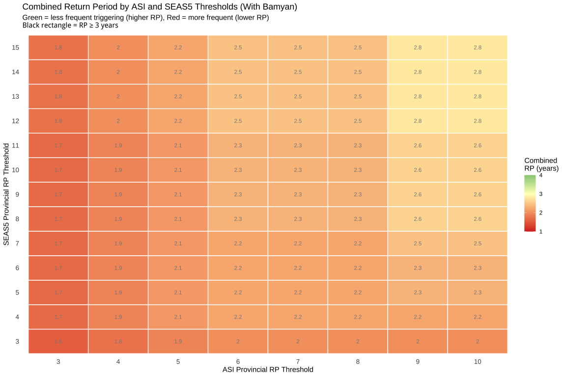
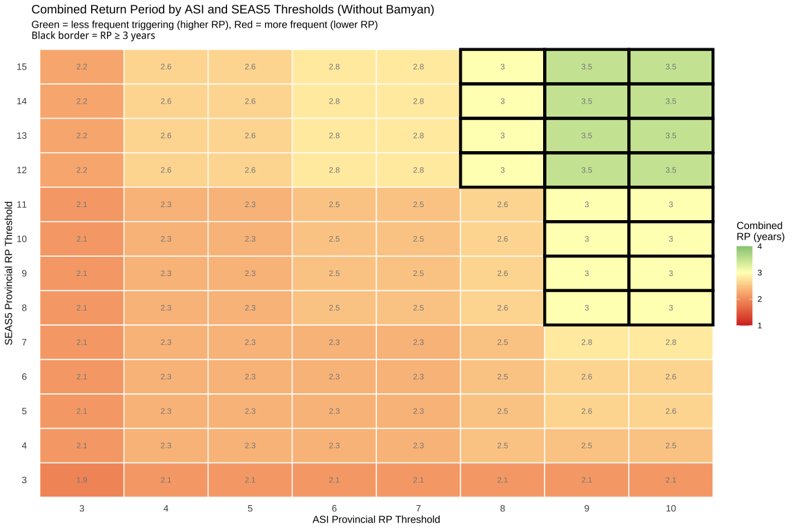
This section examines the effective return period when triggering on ANY province exceeding a threshold. For each provincial RP threshold (3-10 years), we determine which years had at least one province exceed that threshold, then empirically calculate the overall return period of that combined event.

This answers the question: “If we activate when any province crosses RP X, how often does that combined trigger fire?”

Code
# Define thresholds to evaluate
rp_thresholds <- 3:10

# Function to calculate combined RP for a given province set
calculate_combined_rp <- function(df_rp, thresholds = 3:10) {

    # For each threshold, determine years with any province exceeding
    map_dfr(thresholds, ~{
        threshold <- .x

        # Flag years where any province exceeds this threshold
        df_year_flags <- df_rp |>
            mutate(exceeds = rp >= threshold) |>
            group_by(year) |>
            summarise(
                any_exceeds = any(exceeds),
                n_provinces_exceeding = sum(exceeds),
                provinces_exceeding = paste(province[exceeds], collapse = ", "),
                .groups = "drop"
            )

        # Count years with any exceedance
        n_years_total <- nrow(df_year_flags)
        n_years_exceeding <- sum(df_year_flags$any_exceeds)

        # Calculate empirical combined RP
        # RP = total years / number of exceedances
        combined_rp <- if (n_years_exceeding > 0) {
            n_years_total / n_years_exceeding
        } else {
            Inf
        }

        tibble(
            provincial_rp_threshold = threshold,
            n_years_total = n_years_total,
            n_years_any_exceeds = n_years_exceeding,
            pct_years_exceeding = round(100 * n_years_exceeding / n_years_total, 1),
            combined_rp_empirical = round(combined_rp, 2)
        )
    })
}
# Calculate combined RP for both province sets
combined_rp_results <- map(df_asi_rp_list, ~{
    calculate_combined_rp(.x, thresholds = rp_thresholds)
})

A.13.1 Combined RP Results - With Bamyan

Code
combined_rp_results$with_bamyan
# A tibble: 8 × 5
  provincial_rp_threshold n_years_total n_years_any_exceeds pct_years_exceeding
                    <int>         <int>               <int>               <dbl>
1                       3            42                  23                54.8
2                       4            42                  20                47.6
3                       5            42                  17                40.5
4                       6            42                  15                35.7
5                       7            42                  14                33.3
6                       8            42                  14                33.3
7                       9            42                  12                28.6
8                      10            42                  12                28.6
# ℹ 1 more variable: combined_rp_empirical <dbl>

A.13.2 Combined RP Results - Without Bamyan

Code
combined_rp_results$without_bamyan
# A tibble: 8 × 5
  provincial_rp_threshold n_years_total n_years_any_exceeds pct_years_exceeding
                    <int>         <int>               <int>               <dbl>
1                       3            42                  18                42.9
2                       4            42                  15                35.7
3                       5            42                  14                33.3
4                       6            42                  13                31  
5                       7            42                  12                28.6
6                       8            42                  11                26.2
7                       9            42                   9                21.4
8                      10            42                   9                21.4
# ℹ 1 more variable: combined_rp_empirical <dbl>

A.13.3 Comparison Plot

Code
# Combine results for plotting
df_combined_rp_plot <- bind_rows(
    combined_rp_results$with_bamyan |> mutate(province_set = "With Bamyan (6 provinces)"),
    combined_rp_results$without_bamyan |> mutate(province_set = "Without Bamyan (5 provinces)")
)

# Function to find x value where line crosses target y (linear interpolation)
find_intersection <- function(df, target_y) {
    # Find the two points bracketing the target
    df_sorted <- df |> arrange(provincial_rp_threshold)

    for (i in 1:(nrow(df_sorted) - 1)) {
        y1 <- df_sorted$combined_rp_empirical[i]
        y2 <- df_sorted$combined_rp_empirical[i + 1]

        if ((y1 <= target_y & y2 >= target_y) | (y1 >= target_y & y2 <= target_y)) {
            x1 <- df_sorted$provincial_rp_threshold[i]
            x2 <- df_sorted$provincial_rp_threshold[i + 1]
            # Linear interpolation
            x_intersect <- x1 + (target_y - y1) * (x2 - x1) / (y2 - y1)
            return(x_intersect)
        }
    }
    return(NA)
}

# Find intersections for both province sets at y=3 and y=4
intersections <- df_combined_rp_plot |>
    group_by(province_set) |>
    group_split() |>
    map_dfr(~{
        tibble(
            province_set = unique(.x$province_set),
            y3_x = find_intersection(.x, 3),
            y4_x = find_intersection(.x, 4)
        )
    })

# Create labels dataframe for intersection points
df_intersect_labels <- bind_rows(
    intersections |>
        filter(!is.na(y3_x)) |>
        transmute(province_set, x = y3_x, y = 3, label = round(y3_x, 1)),
    intersections |>
        filter(!is.na(y4_x)) |>
        transmute(province_set, x = y4_x, y = 4, label = round(y4_x, 1))
)

ggplot(
    df_combined_rp_plot,
    aes(x = provincial_rp_threshold, y = combined_rp_empirical, color = province_set)
) +
    geom_line(linewidth = 1) +
    geom_point(size = 3) +
    geom_hline(yintercept = 3, linetype = "dashed", color = "gray40", linewidth = 0.8) +
    geom_hline(yintercept = 4, linetype = "dashed", color = "gray40", linewidth = 0.8) +
    geom_point(
        data = df_intersect_labels,
        aes(x = x, y = y),
        size = 4, shape = 21, fill = "white", stroke = 1.5,
        show.legend = FALSE
    ) +
    geom_label(
        data = df_intersect_labels,
        aes(x = x, y = y, label = label),
        vjust = -1, size = 3.5, fontface = "bold",
        label.size = 0.3,
        show.legend = FALSE
    ) +
    annotate("text", x = 1, y = 3, label = "3-yr RP", hjust = 0, vjust = -0.5, size = 3, color = "gray30") +
    annotate("text", x = 1, y = 4, label = "4-yr RP", hjust = 0, vjust = -0.5, size = 3, color = "gray30") +
    scale_x_continuous(breaks = seq(2, 20, by = 2), limits = c(NA, 20)) +
    scale_y_continuous(breaks = seq(0, 10, by = 1)) +
    labs(
        title = "Combined Return Period vs Provincial Threshold",
        subtitle = "Empirical RP when ANY province exceeds the threshold\nHorizontal dashed lines at 3 and 4 year combined RP targets",
        x = "Provincial RP Threshold (years)",
        y = "Combined Empirical RP (years)",
        color = "Province Set"
    ) +
    theme(legend.position = "bottom")

A.13.4 Detailed Year-by-Year Exceedances

Code
# Function to get detailed yearly exceedances
get_yearly_exceedance_detail <- function(df_rp, thresholds = c(3, 5, 7, 10)) {

    map_dfr(thresholds, ~{
        threshold <- .x

        df_rp |>
            mutate(exceeds = rp >= threshold) |>
            group_by(year) |>
            summarise(
                n_provinces_exceeding = sum(exceeds),
                provinces_exceeding = paste(province[exceeds], collapse = ", "),
                .groups = "drop"
            ) |>
            filter(n_provinces_exceeding > 0) |>
            mutate(rp_threshold = threshold) |>
            select(rp_threshold, year, n_provinces_exceeding, provinces_exceeding)
    })
}
# Show detail for key thresholds (with Bamyan)
cat("Years with threshold exceedances (With Bamyan):\n\n")
Years with threshold exceedances (With Bamyan):
Code
get_yearly_exceedance_detail(df_asi_rp_list$with_bamyan) |>
    arrange(rp_threshold, year) |>
    print(n = 50)
# A tibble: 66 × 4
   rp_threshold  year n_provinces_exceeding provinces_exceeding                 
          <dbl> <dbl>                 <int> <chr>                               
 1            3  1985                     4 Badghis, Bamyan, Jawzjan, Sar-e-Pul 
 2            3  1986                     5 Balkh, Bamyan, Faryab, Jawzjan, Sar…
 3            3  1987                     1 Bamyan                              
 4            3  1989                     5 Balkh, Bamyan, Faryab, Jawzjan, Sar…
 5            3  1990                     4 Balkh, Bamyan, Faryab, Sar-e-Pul    
 6            3  1991                     1 Bamyan                              
 7            3  1995                     1 Bamyan                              
 8            3  1996                     1 Bamyan                              
 9            3  1997                     1 Bamyan                              
10            3  2000                     1 Badghis                             
11            3  2001                     6 Badghis, Balkh, Bamyan, Faryab, Jaw…
12            3  2004                     5 Badghis, Balkh, Faryab, Jawzjan, Sa…
13            3  2006                     5 Badghis, Balkh, Bamyan, Faryab, Sar…
14            3  2007                     6 Badghis, Balkh, Bamyan, Faryab, Jaw…
15            3  2008                     6 Badghis, Balkh, Bamyan, Faryab, Jaw…
16            3  2011                     5 Badghis, Balkh, Faryab, Jawzjan, Sa…
17            3  2017                     1 Badghis                             
18            3  2018                     5 Badghis, Balkh, Faryab, Jawzjan, Sa…
19            3  2021                     5 Badghis, Balkh, Faryab, Jawzjan, Sa…
20            3  2022                     6 Badghis, Balkh, Bamyan, Faryab, Jaw…
21            3  2023                     4 Badghis, Balkh, Faryab, Jawzjan     
22            3  2024                     1 Jawzjan                             
23            3  2025                     5 Badghis, Balkh, Faryab, Jawzjan, Sa…
24            5  1985                     1 Bamyan                              
25            5  1986                     4 Balkh, Bamyan, Jawzjan, Sar-e-Pul   
26            5  1987                     1 Bamyan                              
27            5  1989                     3 Bamyan, Faryab, Sar-e-Pul           
28            5  1990                     2 Bamyan, Sar-e-Pul                   
29            5  1991                     1 Bamyan                              
30            5  2000                     1 Badghis                             
31            5  2001                     6 Badghis, Balkh, Bamyan, Faryab, Jaw…
32            5  2006                     2 Badghis, Balkh                      
33            5  2007                     5 Balkh, Bamyan, Faryab, Jawzjan, Sar…
34            5  2008                     5 Badghis, Balkh, Faryab, Jawzjan, Sa…
35            5  2011                     2 Balkh, Sar-e-Pul                    
36            5  2018                     3 Badghis, Faryab, Jawzjan            
37            5  2021                     2 Badghis, Faryab                     
38            5  2022                     4 Badghis, Faryab, Jawzjan, Sar-e-Pul 
39            5  2023                     2 Balkh, Jawzjan                      
40            5  2025                     4 Badghis, Balkh, Faryab, Jawzjan     
41            7  1985                     1 Bamyan                              
42            7  1986                     3 Balkh, Bamyan, Jawzjan              
43            7  1989                     2 Bamyan, Faryab                      
44            7  1990                     2 Bamyan, Sar-e-Pul                   
45            7  1991                     1 Bamyan                              
46            7  2001                     5 Badghis, Balkh, Faryab, Jawzjan, Sa…
47            7  2007                     4 Balkh, Bamyan, Faryab, Sar-e-Pul    
48            7  2008                     5 Badghis, Balkh, Faryab, Jawzjan, Sa…
49            7  2011                     2 Balkh, Sar-e-Pul                    
50            7  2018                     3 Badghis, Faryab, Jawzjan            
# ℹ 16 more rows
Code
# Show detail for key thresholds (without Bamyan)
cat("Years with threshold exceedances (Without Bamyan):\n\n")
Years with threshold exceedances (Without Bamyan):
Code
get_yearly_exceedance_detail(df_asi_rp_list$without_bamyan) |>
    arrange(rp_threshold, year) |>
    print(n = 50)
# A tibble: 53 × 4
   rp_threshold  year n_provinces_exceeding provinces_exceeding                 
          <dbl> <dbl>                 <int> <chr>                               
 1            3  1985                     3 Badghis, Jawzjan, Sar-e-Pul         
 2            3  1986                     4 Balkh, Faryab, Jawzjan, Sar-e-Pul   
 3            3  1989                     4 Balkh, Faryab, Jawzjan, Sar-e-Pul   
 4            3  1990                     3 Balkh, Faryab, Sar-e-Pul            
 5            3  2000                     1 Badghis                             
 6            3  2001                     5 Badghis, Balkh, Faryab, Jawzjan, Sa…
 7            3  2004                     5 Badghis, Balkh, Faryab, Jawzjan, Sa…
 8            3  2006                     4 Badghis, Balkh, Faryab, Sar-e-Pul   
 9            3  2007                     5 Badghis, Balkh, Faryab, Jawzjan, Sa…
10            3  2008                     5 Badghis, Balkh, Faryab, Jawzjan, Sa…
11            3  2011                     5 Badghis, Balkh, Faryab, Jawzjan, Sa…
12            3  2017                     1 Badghis                             
13            3  2018                     5 Badghis, Balkh, Faryab, Jawzjan, Sa…
14            3  2021                     5 Badghis, Balkh, Faryab, Jawzjan, Sa…
15            3  2022                     5 Badghis, Balkh, Faryab, Jawzjan, Sa…
16            3  2023                     4 Badghis, Balkh, Faryab, Jawzjan     
17            3  2024                     1 Jawzjan                             
18            3  2025                     5 Badghis, Balkh, Faryab, Jawzjan, Sa…
19            5  1986                     3 Balkh, Jawzjan, Sar-e-Pul           
20            5  1989                     2 Faryab, Sar-e-Pul                   
21            5  1990                     1 Sar-e-Pul                           
22            5  2000                     1 Badghis                             
23            5  2001                     5 Badghis, Balkh, Faryab, Jawzjan, Sa…
24            5  2006                     2 Badghis, Balkh                      
25            5  2007                     4 Balkh, Faryab, Jawzjan, Sar-e-Pul   
26            5  2008                     5 Badghis, Balkh, Faryab, Jawzjan, Sa…
27            5  2011                     2 Balkh, Sar-e-Pul                    
28            5  2018                     3 Badghis, Faryab, Jawzjan            
29            5  2021                     2 Badghis, Faryab                     
30            5  2022                     4 Badghis, Faryab, Jawzjan, Sar-e-Pul 
31            5  2023                     2 Balkh, Jawzjan                      
32            5  2025                     4 Badghis, Balkh, Faryab, Jawzjan     
33            7  1986                     2 Balkh, Jawzjan                      
34            7  1989                     1 Faryab                              
35            7  1990                     1 Sar-e-Pul                           
36            7  2001                     5 Badghis, Balkh, Faryab, Jawzjan, Sa…
37            7  2007                     3 Balkh, Faryab, Sar-e-Pul            
38            7  2008                     5 Badghis, Balkh, Faryab, Jawzjan, Sa…
39            7  2011                     2 Balkh, Sar-e-Pul                    
40            7  2018                     3 Badghis, Faryab, Jawzjan            
41            7  2021                     1 Badghis                             
42            7  2022                     2 Badghis, Sar-e-Pul                  
43            7  2023                     1 Jawzjan                             
44            7  2025                     4 Badghis, Balkh, Faryab, Jawzjan     
45           10  1986                     1 Balkh                               
46           10  1990                     1 Sar-e-Pul                           
47           10  2001                     5 Badghis, Balkh, Faryab, Jawzjan, Sa…
48           10  2007                     2 Faryab, Sar-e-Pul                   
49           10  2008                     5 Badghis, Balkh, Faryab, Jawzjan, Sa…
50           10  2011                     1 Balkh                               
# ℹ 3 more rows

A.13.5 Summary Table

Code
# Create a comparison table
df_combined_rp_wide <- df_combined_rp_plot |>
    select(provincial_rp_threshold, province_set, combined_rp_empirical) |>
    pivot_wider(
        names_from = province_set,
        values_from = combined_rp_empirical
    )

df_combined_rp_wide |>
    mutate(
        rp_reduction_pct = round(
            100 * (1 - `With Bamyan (6 provinces)` / `Without Bamyan (5 provinces)`),
            1
        )
    )
# A tibble: 8 × 4
  provincial_rp_threshold `With Bamyan (6 provinces)` Without Bamyan (5 provin…¹
                    <int>                       <dbl>                      <dbl>
1                       3                        1.83                       2.33
2                       4                        2.1                        2.8 
3                       5                        2.47                       3   
4                       6                        2.8                        3.23
5                       7                        3                          3.5 
6                       8                        3                          3.82
7                       9                        3.5                        4.67
8                      10                        3.5                        4.67
# ℹ abbreviated name: ¹​`Without Bamyan (5 provinces)`
# ℹ 1 more variable: rp_reduction_pct <dbl>

The rp_reduction_pct column shows how much more frequently the combined trigger fires when including Bamyan (negative values mean the combined RP is lower/more frequent with Bamyan included).

Code
seas5 <- cumulus::pg_load_seas5_historical(
  iso3 = "afg",
  adm_level = 1,
  adm_name = c(PROVINCES_AOI_WITH_BAMYAN)
)
all(PROVINCES_AOI_WITH_BAMYAN %in% seas5$name)
[1] TRUE
Code
seas5_valid_mam <- cumulus::seas5_aggregate_forecast(df =seas5,
                                  value = "mean",
                                  valid_months = c(3,4,5),
                                   by = c("iso3", "pcode", "name","issued_date")
  )

seas5_moment <- seas5_valid_mam |>
  filter(leadtime==0)

A.14 SEAS5 Rainfall Forecast Analysis

This section calculates return periods for SEAS5 March-published rainfall forecasts (valid for MAM season). Lower rainfall = higher drought risk = higher RP, so we use direction = "1".

Code
# Extract year from issued_date for joining with ASI
df_seas5_rp <- seas5_moment |>
    mutate(
        year = year(issued_date)
    ) |>
    group_by(name) |>
    mutate(
        # direction = "1" means lower values get higher RP
        rp = utils$rp_empirical(x = mean, direction = "1", ties_method = "average")
    ) |>
    ungroup() |>
    rename(province = name)

# View the SEAS5 return periods
df_seas5_rp |>
    select(year, province, mean, rp) |>
    arrange(province, desc(rp)) |>
    print(n = 30)
# A tibble: 270 × 4
    year province  mean    rp
   <dbl> <chr>    <dbl> <dbl>
 1  2004 Badghis   84.0 46   
 2  2001 Badghis   97.0 23   
 3  2008 Badghis  105.  15.3 
 4  1985 Badghis  113.  11.5 
 5  2000 Badghis  114.   9.2 
 6  2006 Badghis  118.   7.67
 7  2010 Badghis  121.   6.57
 8  2021 Badghis  124.   5.75
 9  2018 Badghis  126.   5.11
10  2012 Badghis  135.   4.6 
11  2022 Badghis  136.   4.18
12  2023 Badghis  139.   3.83
13  1990 Badghis  149.   3.54
14  2013 Badghis  151.   3.29
15  2014 Badghis  153.   3.07
16  1981 Badghis  153.   2.88
17  1984 Badghis  157.   2.71
18  2002 Badghis  163.   2.56
19  1986 Badghis  169.   2.42
20  2025 Badghis  169.   2.3 
21  2003 Badghis  173.   2.19
22  2017 Badghis  174.   2.09
23  2011 Badghis  175.   2   
24  1989 Badghis  178.   1.92
25  2024 Badghis  181.   1.84
26  2019 Badghis  182.   1.77
27  1988 Badghis  195.   1.70
28  1994 Badghis  196.   1.64
29  1999 Badghis  196.   1.59
30  1987 Badghis  198.   1.53
# ℹ 240 more rows

A.14.1 SEAS5 Threshold Flags

Code
# Create threshold flags for SEAS5
df_seas5_flags <- df_seas5_rp |>
    mutate(
        flag_rp3 = as.integer(rp >= 3),
        flag_rp4 = as.integer(rp >= 4),
        flag_rp5 = as.integer(rp >= 5)
    )

# Summary of threshold exceedances
df_seas5_flags |>
    group_by(province) |>
    summarise(
        n_years = n(),
        n_rp3 = sum(flag_rp3),
        n_rp4 = sum(flag_rp4),
        n_rp5 = sum(flag_rp5),
        pct_rp3 = round(100 * mean(flag_rp3), 1),
        pct_rp4 = round(100 * mean(flag_rp4), 1),
        pct_rp5 = round(100 * mean(flag_rp5), 1),
        .groups = "drop"
    ) |>
    arrange(province)
# A tibble: 6 × 8
  province  n_years n_rp3 n_rp4 n_rp5 pct_rp3 pct_rp4 pct_rp5
  <chr>       <int> <int> <int> <int>   <dbl>   <dbl>   <dbl>
1 Badghis        45    15    11     9    33.3    24.4      20
2 Balkh          45    15    11     9    33.3    24.4      20
3 Bamyan         45    15    11     9    33.3    24.4      20
4 Faryab         45    15    11     9    33.3    24.4      20
5 Jawzjan        45    15    11     9    33.3    24.4      20
6 Sar-e-Pul      45    15    11     9    33.3    24.4      20

A.14.2 SEAS5 Combined RP (Forecast Only)

Code
# Calculate combined RP for SEAS5 alone
combined_rp_seas5 <- calculate_combined_rp(df_seas5_rp, thresholds = rp_thresholds)

combined_rp_seas5
# A tibble: 8 × 5
  provincial_rp_threshold n_years_total n_years_any_exceeds pct_years_exceeding
                    <int>         <int>               <int>               <dbl>
1                       3            45                  17                37.8
2                       4            45                  14                31.1
3                       5            45                  13                28.9
4                       6            45                  12                26.7
5                       7            45                  11                24.4
6                       8            45                  10                22.2
7                       9            45                  10                22.2
8                      10            45                   8                17.8
# ℹ 1 more variable: combined_rp_empirical <dbl>

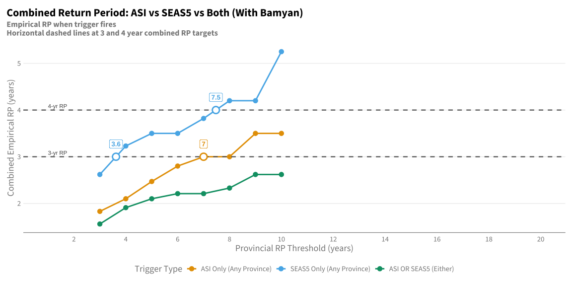
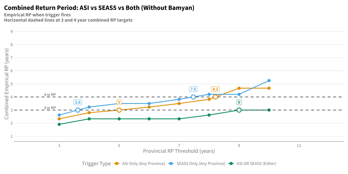
A.15 Combined ASI + SEAS5 Return Period Analysis

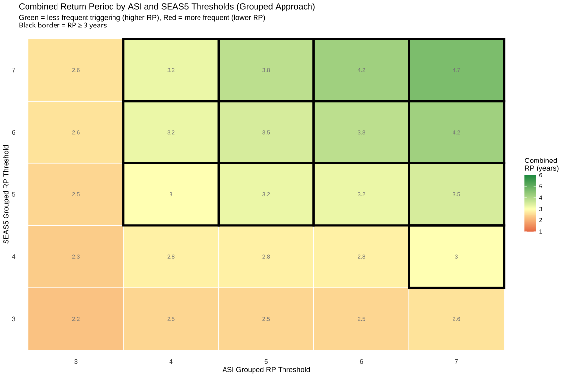
This section examines the effective return period when combining both: 1. ASI observational trigger: ANY province exceeds ASI RP threshold (end of season) 2. SEAS5 forecast trigger: ANY province forecast exceeds rainfall RP threshold (March publication)

We calculate the combined RP when EITHER trigger fires.

Code
# Function to calculate combined RP across ASI and SEAS5
calculate_combined_rp_asi_seas5 <- function(df_asi_rp, df_seas5_rp, thresholds = 3:10) {

    map_dfr(thresholds, ~{
        threshold <- .x

        # Get years where ASI exceeds threshold for any province
        df_asi_years <- df_asi_rp |>
            mutate(exceeds = rp >= threshold) |>
            group_by(year) |>
            summarise(
                asi_any_exceeds = any(exceeds),
                asi_n_provinces = sum(exceeds),
                .groups = "drop"
            )

        # Get years where SEAS5 exceeds threshold for any province
        df_seas5_years <- df_seas5_rp |>
            mutate(exceeds = rp >= threshold) |>
            group_by(year) |>
            summarise(
                seas5_any_exceeds = any(exceeds),
                seas5_n_provinces = sum(exceeds),
                .groups = "drop"
            )

        # Join and calculate combined trigger
        df_combined <- df_asi_years |>
            inner_join(df_seas5_years, by = "year") |>
            mutate(
                either_exceeds = asi_any_exceeds | seas5_any_exceeds,
                both_exceed = asi_any_exceeds & seas5_any_exceeds
            )

        n_years_total <- nrow(df_combined)
        n_asi_only <- sum(df_combined$asi_any_exceeds & !df_combined$seas5_any_exceeds)
        n_seas5_only <- sum(df_combined$seas5_any_exceeds & !df_combined$asi_any_exceeds)
        n_both <- sum(df_combined$both_exceed)
        n_either <- sum(df_combined$either_exceeds)

        tibble(
            provincial_rp_threshold = threshold,
            n_years_total = n_years_total,
            n_asi_only = n_asi_only,
            n_seas5_only = n_seas5_only,
            n_both = n_both,
            n_either = n_either,
            combined_rp_asi_only = round(n_years_total / sum(df_combined$asi_any_exceeds), 2),
            combined_rp_seas5_only = round(n_years_total / sum(df_combined$seas5_any_exceeds), 2),
            combined_rp_either = round(if_else(n_either > 0, n_years_total / n_either, Inf), 2)
        )
    })
}
# Calculate for both province sets
combined_rp_asi_seas5_results <- map(df_asi_rp_list, ~{
    calculate_combined_rp_asi_seas5(.x, df_seas5_rp, thresholds = rp_thresholds)
})

A.15.1 Combined Results - With Bamyan

Code
combined_rp_asi_seas5_results$with_bamyan
# A tibble: 8 × 9
  provincial_rp_threshold n_years_total n_asi_only n_seas5_only n_both n_either
                    <int>         <int>      <int>        <int>  <int>    <int>
1                       3            42         11            4     12       27
2                       4            42          9            2     11       22
3                       5            42          8            3      9       20
4                       6            42          7            4      8       19
5                       7            42          8            5      6       19
6                       8            42          8            4      6       18
7                       9            42          6            4      6       16
8                      10            42          8            4      4       16
# ℹ 3 more variables: combined_rp_asi_only <dbl>, combined_rp_seas5_only <dbl>,
#   combined_rp_either <dbl>

A.15.2 Combined Results - Without Bamyan

Code
combined_rp_asi_seas5_results$without_bamyan
# A tibble: 8 × 9
  provincial_rp_threshold n_years_total n_asi_only n_seas5_only n_both n_either
                    <int>         <int>      <int>        <int>  <int>    <int>
1                       3            42          6            4     12       22
2                       4            42          5            3     10       18
3                       5            42          6            4      8       18
4                       6            42          6            5      7       18
5                       7            42          7            6      5       18
6                       8            42          6            5      5       16
7                       9            42          4            5      5       14
8                      10            42          6            5      3       14
# ℹ 3 more variables: combined_rp_asi_only <dbl>, combined_rp_seas5_only <dbl>,
#   combined_rp_either <dbl>

A.15.3 Comparison Plot: ASI vs SEAS5 vs Combined

Code
# Prepare data for plotting (with Bamyan)
df_plot_combined <- combined_rp_asi_seas5_results$with_bamyan |>
    select(provincial_rp_threshold, combined_rp_asi_only, combined_rp_seas5_only, combined_rp_either) |>
    pivot_longer(
        cols = starts_with("combined_rp"),
        names_to = "trigger_type",
        values_to = "combined_rp"
    ) |>
    mutate(
        trigger_type = case_when(
            trigger_type == "combined_rp_asi_only" ~ "ASI Only (Any Province)",
            trigger_type == "combined_rp_seas5_only" ~ "SEAS5 Only (Any Province)",
            trigger_type == "combined_rp_either" ~ "ASI OR SEAS5 (Either)"
        ),
        trigger_type = factor(trigger_type, levels = c(
            "ASI Only (Any Province)",
            "SEAS5 Only (Any Province)",
            "ASI OR SEAS5 (Either)"
        ))
    )

# Function to find x value where line crosses target y (linear interpolation)
find_intersection_asi_seas5 <- function(df, target_y) {
    df_sorted <- df |> arrange(provincial_rp_threshold)
    for (i in 1:(nrow(df_sorted) - 1)) {
        y1 <- df_sorted$combined_rp[i]
        y2 <- df_sorted$combined_rp[i + 1]
        if ((y1 <= target_y & y2 >= target_y) | (y1 >= target_y & y2 <= target_y)) {
            x1 <- df_sorted$provincial_rp_threshold[i]
            x2 <- df_sorted$provincial_rp_threshold[i + 1]
            x_intersect <- x1 + (target_y - y1) * (x2 - x1) / (y2 - y1)
            return(x_intersect)
        }
    }
    return(NA)
}

# Find intersections for all trigger types at y=3 and y=4
intersections_asi_seas5 <- df_plot_combined |>
    group_by(trigger_type) |>
    group_split() |>
    map_dfr(~{
        tibble(
            trigger_type = unique(.x$trigger_type),
            y3_x = find_intersection_asi_seas5(.x, 3),
            y4_x = find_intersection_asi_seas5(.x, 4)
        )
    })

# Create labels dataframe for intersection points
df_intersect_labels_asi_seas5 <- bind_rows(
    intersections_asi_seas5 |>
        filter(!is.na(y3_x)) |>
        transmute(trigger_type, x = y3_x, y = 3, label = round(y3_x, 1)),
    intersections_asi_seas5 |>
        filter(!is.na(y4_x)) |>
        transmute(trigger_type, x = y4_x, y = 4, label = round(y4_x, 1))
)

ggplot(
    df_plot_combined,
    aes(x = provincial_rp_threshold, y = combined_rp, color = trigger_type)
) +
    geom_line(linewidth = 1) +
    geom_point(size = 3) +
    geom_hline(yintercept = 3, linetype = "dashed", color = "gray40", linewidth = 0.8) +
    geom_hline(yintercept = 4, linetype = "dashed", color = "gray40", linewidth = 0.8) +
    geom_point(
        data = df_intersect_labels_asi_seas5,
        aes(x = x, y = y),
        size = 4, shape = 21, fill = "white", stroke = 1.5,
        show.legend = FALSE
    ) +
    geom_label(
        data = df_intersect_labels_asi_seas5,
        aes(x = x, y = y, label = label),
        vjust = -1, size = 3.5, fontface = "bold",
        label.size = 0.3,
        show.legend = FALSE
    ) +
    annotate("text", x = 1, y = 3, label = "3-yr RP", hjust = 0, vjust = -0.5, size = 3, color = "gray30") +
    annotate("text", x = 1, y = 4, label = "4-yr RP", hjust = 0, vjust = -0.5, size = 3, color = "gray30") +
    scale_x_continuous(breaks = seq(2, 20, by = 2), limits = c(NA, 20)) +
    scale_y_continuous(breaks = seq(0, 10, by = 1)) +
    scale_color_manual(values = c(
        "ASI Only (Any Province)" = "#E69F00",
        "SEAS5 Only (Any Province)" = "#56B4E9",
        "ASI OR SEAS5 (Either)" = "#009E73"
    )) +
    labs(
        title = "Combined Return Period: ASI vs SEAS5 vs Both (With Bamyan)",
        subtitle = "Empirical RP when trigger fires\nHorizontal dashed lines at 3 and 4 year combined RP targets",
        x = "Provincial RP Threshold (years)",
        y = "Combined Empirical RP (years)",
        color = "Trigger Type"
    ) +
    theme(legend.position = "bottom")

Code
# Same plot without Bamyan
df_plot_combined_nb <- combined_rp_asi_seas5_results$without_bamyan |>
    select(provincial_rp_threshold, combined_rp_asi_only, combined_rp_seas5_only, combined_rp_either) |>
    pivot_longer(
        cols = starts_with("combined_rp"),
        names_to = "trigger_type",
        values_to = "combined_rp"
    ) |>
    mutate(
        trigger_type = case_when(
            trigger_type == "combined_rp_asi_only" ~ "ASI Only (Any Province)",
            trigger_type == "combined_rp_seas5_only" ~ "SEAS5 Only (Any Province)",
            trigger_type == "combined_rp_either" ~ "ASI OR SEAS5 (Either)"
        ),
        trigger_type = factor(trigger_type, levels = c(
            "ASI Only (Any Province)",
            "SEAS5 Only (Any Province)",
            "ASI OR SEAS5 (Either)"
        ))
    )

# Find intersections for all trigger types at y=3 and y=4
intersections_nb <- df_plot_combined_nb |>
    group_by(trigger_type) |>
    group_split() |>
    map_dfr(~{
        tibble(
            trigger_type = unique(.x$trigger_type),
            y3_x = find_intersection_asi_seas5(.x, 3),
            y4_x = find_intersection_asi_seas5(.x, 4)
        )
    })

# Create labels dataframe for intersection points
df_intersect_labels_nb <- bind_rows(
    intersections_nb |>
        filter(!is.na(y3_x)) |>
        transmute(trigger_type, x = y3_x, y = 3, label = round(y3_x, 1)),
    intersections_nb |>
        filter(!is.na(y4_x)) |>
        transmute(trigger_type, x = y4_x, y = 4, label = round(y4_x, 1))
)

ggplot(
    df_plot_combined_nb,
    aes(x = provincial_rp_threshold, y = combined_rp, color = trigger_type)
) +
    geom_line(linewidth = 1) +
    geom_point(size = 3) +
    geom_hline(yintercept = 3, linetype = "dashed", color = "gray40", linewidth = 0.8) +
    geom_hline(yintercept = 4, linetype = "dashed", color = "gray40", linewidth = 0.8) +
    geom_point(
        data = df_intersect_labels_nb,
        aes(x = x, y = y),
        size = 4, shape = 21, fill = "white", stroke = 1.5,
        show.legend = FALSE
    ) +
    geom_label(
        data = df_intersect_labels_nb,
        aes(x = x, y = y, label = label),
        vjust = -1, size = 3.5, fontface = "bold",
        label.size = 0.3,
        show.legend = FALSE
    ) +
    annotate("text", x = 2.5, y = 3, label = "3-yr RP", hjust = 0, vjust = -0.5, size = 3, color = "gray30") +
    annotate("text", x = 2.5, y = 4, label = "4-yr RP", hjust = 0, vjust = -0.5, size = 3, color = "gray30") +
    scale_x_continuous(breaks = seq(3, 12, by = 2), limits = c(2, 12)) +
    scale_y_continuous(breaks = seq(1, 9, by = 1), limits = c(1, 9)) +
    scale_color_manual(values = c(
        "ASI Only (Any Province)" = "#E69F00",
        "SEAS5 Only (Any Province)" = "#56B4E9",
        "ASI OR SEAS5 (Either)" = "#009E73"
    )) +
    labs(
        title = "Combined Return Period: ASI vs SEAS5 vs Both (Without Bamyan)",
        subtitle = "Empirical RP when trigger fires\nHorizontal dashed lines at 3 and 4 year combined RP targets",
        x = "Provincial RP Threshold (years)",
        y = "Combined Empirical RP (years)",
        color = "Trigger Type"
    ) +
    theme(legend.position = "bottom")

A.15.4 Year-by-Year Trigger Comparison

Code
# Detailed year-by-year comparison at key thresholds
get_yearly_trigger_detail <- function(df_asi_rp, df_seas5_rp, threshold = 5) {

    df_asi <- df_asi_rp |>
        mutate(asi_exceeds = rp >= threshold) |>
        group_by(year) |>
        summarise(
            asi_triggered = any(asi_exceeds),
            asi_provinces = paste(province[asi_exceeds], collapse = ", "),
            .groups = "drop"
        )

    df_seas5 <- df_seas5_rp |>
        mutate(seas5_exceeds = rp >= threshold) |>
        group_by(year) |>
        summarise(
            seas5_triggered = any(seas5_exceeds),
            seas5_provinces = paste(province[seas5_exceeds], collapse = ", "),
            .groups = "drop"
        )

    df_asi |>
        inner_join(df_seas5, by = "year") |>
        filter(asi_triggered | seas5_triggered) |>
        mutate(
            trigger_type = case_when(
                asi_triggered & seas5_triggered ~ "Both",
                asi_triggered ~ "ASI Only",
                seas5_triggered ~ "SEAS5 Only"
            )
        ) |>
        select(year, trigger_type, asi_provinces, seas5_provinces)
}

# Show detail for 5-year RP threshold
cat("Years triggering at 5-Year RP Threshold (With Bamyan):\n\n")
Years triggering at 5-Year RP Threshold (With Bamyan):
Code
get_yearly_trigger_detail(df_asi_rp_list$with_bamyan, df_seas5_rp, threshold = 5) |>
    print(n = 30)
# A tibble: 20 × 4
    year trigger_type asi_provinces                              seas5_provinces
   <dbl> <chr>        <chr>                                      <chr>          
 1  1985 Both         "Bamyan"                                   "Bamyan, Sar-e…
 2  1986 ASI Only     "Balkh, Bamyan, Jawzjan, Sar-e-Pul"        ""             
 3  1987 ASI Only     "Bamyan"                                   ""             
 4  1989 ASI Only     "Bamyan, Faryab, Sar-e-Pul"                ""             
 5  1990 Both         "Bamyan, Sar-e-Pul"                        "Bamyan, Balkh…
 6  1991 ASI Only     "Bamyan"                                   ""             
 7  2000 Both         "Badghis"                                  "Balkh, Sar-e-…
 8  2001 Both         "Badghis, Balkh, Bamyan, Faryab, Jawzjan,… "Balkh, Sar-e-…
 9  2004 SEAS5 Only   ""                                         "Bamyan, Balkh…
10  2006 Both         "Badghis, Balkh"                           "Bamyan, Balkh…
11  2007 ASI Only     "Balkh, Bamyan, Faryab, Jawzjan, Sar-e-Pu… ""             
12  2008 Both         "Badghis, Balkh, Faryab, Jawzjan, Sar-e-P… "Bamyan, Balkh…
13  2010 SEAS5 Only   ""                                         "Bamyan, Sar-e…
14  2011 ASI Only     "Balkh, Sar-e-Pul"                         ""             
15  2012 SEAS5 Only   ""                                         "Bamyan, Balkh…
16  2018 Both         "Badghis, Faryab, Jawzjan"                 "Bamyan, Balkh…
17  2021 Both         "Badghis, Faryab"                          "Jawzjan, Fary…
18  2022 ASI Only     "Badghis, Faryab, Jawzjan, Sar-e-Pul"      ""             
19  2023 Both         "Balkh, Jawzjan"                           "Balkh, Jawzja…
20  2025 ASI Only     "Badghis, Balkh, Faryab, Jawzjan"          ""             

A.15.5 Summary Comparison Table

Code
# Create summary comparison
df_summary <- combined_rp_asi_seas5_results$with_bamyan |>
    select(
        provincial_rp_threshold,
        n_years_total,
        n_asi_only,
        n_seas5_only,
        n_both,
        n_either,
        combined_rp_asi_only,
        combined_rp_seas5_only,
        combined_rp_either
    ) |>
    mutate(
        rp_reduction_pct = round(
            100 * (1 - combined_rp_either / combined_rp_asi_only),
            1
        )
    )

df_summary
# A tibble: 8 × 10
  provincial_rp_threshold n_years_total n_asi_only n_seas5_only n_both n_either
                    <int>         <int>      <int>        <int>  <int>    <int>
1                       3            42         11            4     12       27
2                       4            42          9            2     11       22
3                       5            42          8            3      9       20
4                       6            42          7            4      8       19
5                       7            42          8            5      6       19
6                       8            42          8            4      6       18
7                       9            42          6            4      6       16
8                      10            42          8            4      4       16
# ℹ 4 more variables: combined_rp_asi_only <dbl>, combined_rp_seas5_only <dbl>,
#   combined_rp_either <dbl>, rp_reduction_pct <dbl>

The rp_reduction_pct shows how much more frequently the combined trigger (ASI OR SEAS5) fires compared to ASI alone. Higher values indicate the forecast adds more “triggering power”.

A.16 Threshold Optimization: Targeting Combined RP

This section explores different combinations of ASI and SEAS5 thresholds to achieve a target combined RP of 3-5 years. The key insight is that we can use different thresholds for each indicator - for example, keeping ASI close to our target while using a higher SEAS5 threshold to reduce false positives from the forecast.

Code
# Define threshold ranges to explore
asi_thresholds <- 3:10
seas5_thresholds <- 3:15

# Function to calculate combined RP for specific ASI and SEAS5 thresholds
calculate_combined_rp_grid <- function(df_asi_rp, df_seas5_rp,
                                        asi_thresholds, seas5_thresholds) {

    # Pre-calculate year-level exceedances for each threshold
    asi_year_flags <- map(asi_thresholds, ~{
        threshold <- .x
        df_asi_rp |>
            mutate(exceeds = rp >= threshold) |>
            group_by(year) |>
            summarise(asi_exceeds = any(exceeds), .groups = "drop")
    }) |>
        set_names(asi_thresholds)

    seas5_year_flags <- map(seas5_thresholds, ~{
        threshold <- .x
        df_seas5_rp |>
            mutate(exceeds = rp >= threshold) |>
            group_by(year) |>
            summarise(seas5_exceeds = any(exceeds), .groups = "drop")
    }) |>
        set_names(seas5_thresholds)

    # Calculate combined RP for each combination
    expand_grid(
        asi_threshold = asi_thresholds,
        seas5_threshold = seas5_thresholds
    ) |>
        pmap_dfr(function(asi_threshold, seas5_threshold) {
            df_combined <- asi_year_flags[[as.character(asi_threshold)]] |>
                inner_join(
                    seas5_year_flags[[as.character(seas5_threshold)]],
                    by = "year"
                ) |>
                mutate(either_exceeds = asi_exceeds | seas5_exceeds)

            n_years <- nrow(df_combined)
            n_asi <- sum(df_combined$asi_exceeds)
            n_seas5 <- sum(df_combined$seas5_exceeds)
            n_either <- sum(df_combined$either_exceeds)

            tibble(
                asi_threshold = asi_threshold,
                seas5_threshold = seas5_threshold,
                n_years = n_years,
                n_asi_fires = n_asi,
                n_seas5_fires = n_seas5,
                n_either_fires = n_either,
                rp_asi = round(n_years / n_asi, 2),
                rp_seas5 = round(n_years / n_seas5, 2),
                rp_combined = round(if_else(n_either > 0, n_years / n_either, Inf), 2)
            )
        })
}
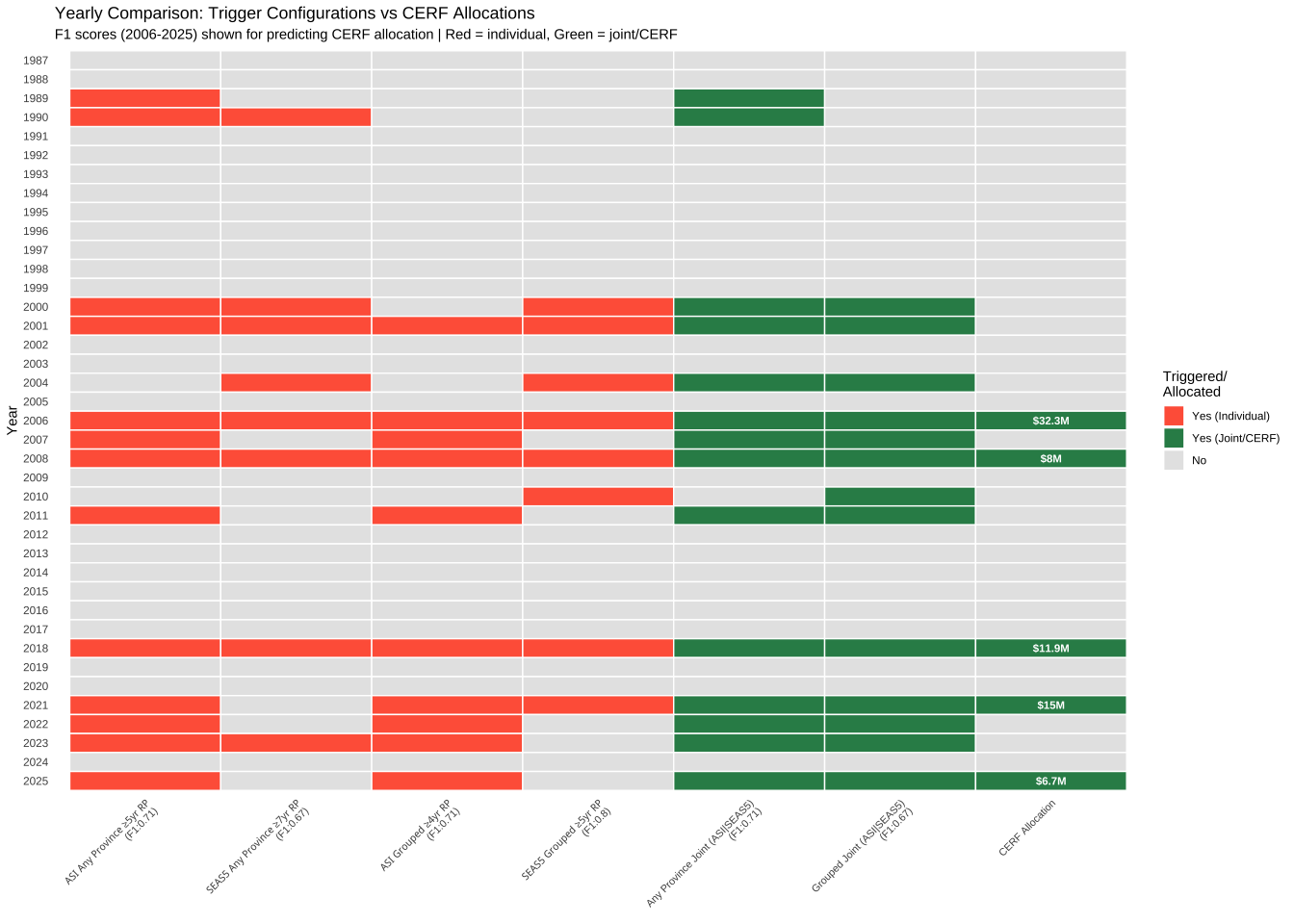
# Calculate grid for both province sets
rp_grid_with_bamyan <- calculate_combined_rp_grid(
    df_asi_rp_list$with_bamyan,
    df_seas5_rp,
    asi_thresholds,
    seas5_thresholds
)

rp_grid_without_bamyan <- calculate_combined_rp_grid(
    df_asi_rp_list$without_bamyan,
    df_seas5_rp,
    asi_thresholds,
    seas5_thresholds
)

A.16.1 Heatmap: Combined RP by Threshold Combination (With Bamyan)

Code
# Find the boundary for RP >= 3
# Get the factor levels to map thresholds to positions
asi_levels <- sort(unique(rp_grid_with_bamyan$asi_threshold))
seas5_levels <- sort(unique(rp_grid_with_bamyan$seas5_threshold))

# Find minimum thresholds that achieve RP >= 3
tiles_over_3 <- rp_grid_with_bamyan |>
    filter(rp_combined >= 3)

# Get the minimum position (lower-left corner of the region)
min_asi_pos <- which(asi_levels == min(tiles_over_3$asi_threshold)) - 0.5
min_seas5_pos <- which(seas5_levels == min(tiles_over_3$seas5_threshold)) - 0.5

# Max positions (upper-right corner)
max_asi_pos <- length(asi_levels) + 0.5
max_seas5_pos <- length(seas5_levels) + 0.5

ggplot(
    rp_grid_with_bamyan,
    aes(x = factor(asi_threshold), y = factor(seas5_threshold), fill = rp_combined)
) +
    geom_tile(color = "white", linewidth = 0.5) +
    geom_text(aes(label = round(rp_combined, 1)), size = 3) +
    annotate(
        "rect",
        xmin = min_asi_pos, xmax = max_asi_pos,
        ymin = min_seas5_pos, ymax = max_seas5_pos,
        fill = NA, color = "black", linewidth = 2, linetype = "solid"
    ) +
    scale_fill_gradient2(
        low = "#d73027",
        mid = "#ffffbf",
        high = "#1a9850",
        midpoint = 3,
        limits = c(1, 4),
        oob = scales::squish,
        name = "Combined\nRP (years)"
    ) +
    labs(
        title = "Combined Return Period by ASI and SEAS5 Thresholds (With Bamyan)",
        subtitle = "Green = less frequent triggering (higher RP), Red = more frequent (lower RP)\nBlack rectangle = RP ≥ 3 years",
        x = "ASI Provincial RP Threshold",
        y = "SEAS5 Provincial RP Threshold"
    ) +
    theme_minimal() +
    theme(
        panel.grid = element_blank(),
        axis.text = element_text(size = 10)
    )

A.16.2 Heatmap: Combined RP by Threshold Combination (Without Bamyan)

Code
# Filter tiles with RP >= 3 for border highlighting
tiles_over_3_nb <- rp_grid_without_bamyan |>
    filter(rp_combined >= 3)

ggplot(
    rp_grid_without_bamyan,
    aes(x = factor(asi_threshold), y = factor(seas5_threshold), fill = rp_combined)
) +
    geom_tile(color = "white", linewidth = 0.5) +
    geom_tile(
        data = tiles_over_3_nb,
        aes(x = factor(asi_threshold), y = factor(seas5_threshold)),
        fill = NA, color = "black", linewidth = 1.5
    ) +
    geom_text(aes(label = round(rp_combined, 1)), size = 3) +
    scale_fill_gradient2(
        low = "#d73027",
        mid = "#ffffbf",
        high = "#1a9850",
        midpoint = 3,
        limits = c(1, 4),
        oob = scales::squish,
        name = "Combined\nRP (years)"
    ) +
    labs(
        title = "Combined Return Period by ASI and SEAS5 Thresholds (Without Bamyan)",
        subtitle = "Green = less frequent triggering (higher RP), Red = more frequent (lower RP)\nBlack border = RP ≥ 3 years",
        x = "ASI Provincial RP Threshold",
        y = "SEAS5 Provincial RP Threshold"
    ) +
    theme_minimal() +
    theme(
        panel.grid = element_blank(),
        axis.text = element_text(size = 10)
    )

A.17 Grouped Analysis - Area-Weighted Provincial Aggregate

This section presents an alternative approach: instead of triggering when ANY province exceeds a threshold, we calculate an area-weighted average across all 5 provinces (without Bamyan) and determine when that grouped value exceeds thresholds. This approach reflects more widespread drought conditions across the region.

We use SEAS5 pixel counts (n_upsampled_pixels) as a proxy for provincial area to weight the averaging.

Code
# Get pixel counts for area weighting
conn <- cumulus::pg_con()
df_pixels <- dplyr::tbl(conn, "polygon") |>
    filter(
        iso3 == "AFG",
        adm_level == 1,
        name %in% PROVINCES_AOI_NO_BAMYAN
    ) |>
    select(
        province = name,
        n_pixels = seas5_n_upsampled_pixels
    ) |>
    collect()

# Grouped ASI (area-weighted average)
df_asi_grouped <- df_asi_eos |>
    filter(province %in% PROVINCES_AOI_NO_BAMYAN) |>
    left_join(df_pixels, by = "province") |>
    group_by(year) |>
    summarise(
        asi_grouped = weighted.mean(data, w = n_pixels, na.rm = TRUE),
        .groups = "drop"
    ) |>
    mutate(
        rp = utils$rp_empirical(x = asi_grouped, direction = "-1", ties_method = "average")
    )

# Grouped SEAS5 (area-weighted average)
df_pixels_seas5 <- df_pixels |> rename(name = province)

df_seas5_grouped <- seas5_moment |>
    filter(name %in% PROVINCES_AOI_NO_BAMYAN) |>
    left_join(df_pixels_seas5, by = "name") |>
    mutate(year = year(issued_date)) |>
    group_by(year) |>
    summarise(
        seas5_grouped = weighted.mean(mean, w = n_pixels, na.rm = TRUE),
        .groups = "drop"
    ) |>
    mutate(
        rp = utils$rp_empirical(x = seas5_grouped, direction = "1", ties_method = "average")
    )

# Combined grouped data
df_grouped_combined <- df_asi_grouped |>
    select(year, asi_rp = rp) |>
    inner_join(
        df_seas5_grouped |> select(year, seas5_rp = rp),
        by = "year"
    )

A.17.1 Heatmap: Combined RP by Threshold Combination (Grouped Approach)

This heatmap shows the combined return period for different combinations of ASI and SEAS5 thresholds using the grouped (area-weighted) approach. The trigger fires when EITHER the grouped ASI OR grouped SEAS5 exceeds its respective threshold.

Code
# Define threshold ranges
asi_thresholds_grouped <- 3:7
seas5_thresholds_grouped <- 3:7

# Calculate combined RP for each threshold combination using grouped data
rp_grid_grouped <- expand_grid(
    asi_threshold = asi_thresholds_grouped,
    seas5_threshold = seas5_thresholds_grouped
) |>
    pmap_dfr(function(asi_threshold, seas5_threshold) {
        n_either <- df_grouped_combined |>
            filter(asi_rp >= asi_threshold | seas5_rp >= seas5_threshold) |>
            nrow()

        n_asi <- sum(df_grouped_combined$asi_rp >= asi_threshold)
        n_seas5 <- sum(df_grouped_combined$seas5_rp >= seas5_threshold)

        total_years <- nrow(df_grouped_combined)

        tibble(
            asi_threshold = asi_threshold,
            seas5_threshold = seas5_threshold,
            n_years = total_years,
            n_asi_fires = n_asi,
            n_seas5_fires = n_seas5,
            n_either_fires = n_either,
            rp_combined = if(n_either > 0) round(total_years / n_either, 2) else Inf
        )
    })

# Filter tiles with RP >= 3 for border highlighting
tiles_over_3_grouped <- rp_grid_grouped |>
    filter(rp_combined >= 3)

ggplot(
    rp_grid_grouped,
    aes(x = factor(asi_threshold), y = factor(seas5_threshold), fill = rp_combined)
) +
    geom_tile(color = "white", linewidth = 0.5) +
    geom_tile(
        data = tiles_over_3_grouped,
        aes(x = factor(asi_threshold), y = factor(seas5_threshold)),
        fill = NA, color = "black", linewidth = 1.5
    ) +
    geom_text(aes(label = round(rp_combined, 1)), size = 3) +
    scale_fill_gradient2(
        low = "#d73027",
        mid = "#ffffbf",
        high = "#1a9850",
        midpoint = 3,
        limits = c(1, 6),
        oob = scales::squish,
        name = "Combined\nRP (years)"
    ) +
    labs(
        title = "Combined Return Period by ASI and SEAS5 Thresholds (Grouped Approach)",
        subtitle = "Green = less frequent triggering (higher RP), Red = more frequent (lower RP)\nBlack border = RP ≥ 3 years",
        x = "ASI Grouped RP Threshold",
        y = "SEAS5 Grouped RP Threshold"
    ) +
    theme_minimal() +
    theme(
        panel.grid = element_blank(),
        axis.text = element_text(size = 10)
    )

A.18 Yearly Comparison to CERF

This section compares different trigger configurations against historical CERF drought allocations to Afghanistan.

Code
# Get overlapping years for comparison (CERF data loaded at top of script)
years_compare <- 1987:2025  # SEAS5 starts 1987

# Build comparison dataframe
df_yearly_comparison <- tibble(year = years_compare) |>
    # ANY province ASI >= 5-year RP
    left_join(
        df_asi_rp_list$without_bamyan |>
            group_by(year) |>
            summarise(asi_any_5yr = any(rp >= 5), .groups = "drop"),
        by = "year"
    ) |>
    # ANY province SEAS5 >= 7-year RP
    left_join(
        df_seas5_rp |>
            filter(province %in% PROVINCES_AOI_NO_BAMYAN) |>
            group_by(year) |>
            summarise(seas5_any_7yr = any(rp >= 7), .groups = "drop"),
        by = "year"
    ) |>
    # Grouped ASI >= 4-year RP
    left_join(
        df_asi_grouped |>
            transmute(year, asi_grouped_4yr = rp >= 4),
        by = "year"
    ) |>
    # Grouped SEAS5 >= 5-year RP
    left_join(
        df_seas5_grouped |>
            transmute(year, seas5_grouped_5yr = rp >= 5),
        by = "year"
    ) |>
    # CERF allocations
    left_join(df_cerf_yearly, by = "year") |>
    mutate(
        cerf_allocation = !is.na(cerf_amount),
        cerf_amount = replace_na(cerf_amount, 0),
        across(c(asi_any_5yr, seas5_any_7yr, asi_grouped_4yr, seas5_grouped_5yr), ~replace_na(.x, FALSE)),
        # Joint triggers (either must fire)
        any_joint = asi_any_5yr | seas5_any_7yr,
        grouped_joint = asi_grouped_4yr | seas5_grouped_5yr
    )
Code
# Calculate precision/recall/F1 for each indicator (2006-2025)
df_metrics_input <- df_yearly_comparison |>
    filter(year >= 2006, year <= 2025)

calc_metrics <- function(predicted, actual) {
    tp <- sum(predicted & actual)
    fp <- sum(predicted & !actual)
    fn <- sum(!predicted & actual)

    precision <- if ((tp + fp) > 0) tp / (tp + fp) else NA
    recall <- if ((tp + fn) > 0) tp / (tp + fn) else NA
    f1 <- if (!is.na(precision) & !is.na(recall) & (precision + recall) > 0) {
        2 * precision * recall / (precision + recall)
    } else NA

    tibble(precision = precision, recall = recall, f1 = f1)
}

df_metrics <- tibble(
    indicator_var = c("asi_any_5yr", "seas5_any_7yr", "asi_grouped_4yr", "seas5_grouped_5yr", "any_joint", "grouped_joint"),
    indicator_label = c(
        "ASI Any Province ≥5yr RP",
        "SEAS5 Any Province ≥7yr RP",
        "ASI Grouped ≥4yr RP",
        "SEAS5 Grouped ≥5yr RP",
        "Any Province Joint (ASI|SEAS5)",
        "Grouped Joint (ASI|SEAS5)"
    )
) |>
    rowwise() |>
    mutate(
        metrics = list(calc_metrics(
            df_metrics_input[[indicator_var]],
            df_metrics_input$cerf_allocation
        ))
    ) |>
    unnest(metrics) |>
    ungroup() |>
    mutate(
        label_with_metrics = paste0(
            indicator_label, "\n",
            "P:", round(precision, 2), " R:", round(recall, 2), " F1:", round(f1, 2)
        )
    )

# Display metrics table
df_metrics |>
    select(indicator_label, precision, recall, f1) |>
    mutate(across(c(precision, recall, f1), ~round(.x, 3)))
# A tibble: 6 × 4
  indicator_label                precision recall    f1
  <chr>                              <dbl>  <dbl> <dbl>
1 ASI Any Province ≥5yr RP           0.556    1   0.714
2 SEAS5 Any Province ≥7yr RP         0.75     0.6 0.667
3 ASI Grouped ≥4yr RP                0.556    1   0.714
4 SEAS5 Grouped ≥5yr RP              0.8      0.8 0.8  
5 Any Province Joint (ASI|SEAS5)     0.556    1   0.714
6 Grouped Joint (ASI|SEAS5)          0.5      1   0.667
Code
# Create label lookup for indicators with metrics
label_lookup <- df_metrics |>
    select(indicator_label, label_with_metrics) |>
    deframe()

# Add CERF (no metrics for itself)
label_lookup["CERF Allocation"] <- "CERF Allocation"

# Prepare data for heatmap (full historical record)
df_heatmap <- df_yearly_comparison |>
    filter(year >= 1987) |>  # Full SEAS5 record
    select(year, asi_any_5yr, seas5_any_7yr, asi_grouped_4yr, seas5_grouped_5yr, any_joint, grouped_joint, cerf_allocation) |>
    pivot_longer(
        cols = -year,
        names_to = "indicator",
        values_to = "triggered"
    ) |>
    mutate(
        indicator = case_when(
            indicator == "asi_any_5yr" ~ "ASI Any Province ≥5yr RP",
            indicator == "seas5_any_7yr" ~ "SEAS5 Any Province ≥7yr RP",
            indicator == "asi_grouped_4yr" ~ "ASI Grouped ≥4yr RP",
            indicator == "seas5_grouped_5yr" ~ "SEAS5 Grouped ≥5yr RP",
            indicator == "any_joint" ~ "Any Province Joint (ASI|SEAS5)",
            indicator == "grouped_joint" ~ "Grouped Joint (ASI|SEAS5)",
            indicator == "cerf_allocation" ~ "CERF Allocation"
        ),
        indicator = factor(indicator, levels = c(
            "ASI Any Province ≥5yr RP",
            "SEAS5 Any Province ≥7yr RP",
            "ASI Grouped ≥4yr RP",
            "SEAS5 Grouped ≥5yr RP",
            "Any Province Joint (ASI|SEAS5)",
            "Grouped Joint (ASI|SEAS5)",
            "CERF Allocation"
        )),
        # Create fill groups: individual indicators (red) vs joint/cerf (green)
        is_joint_or_cerf = indicator %in% c(
            "Any Province Joint (ASI|SEAS5)",
            "Grouped Joint (ASI|SEAS5)",
            "CERF Allocation"
        ),
        fill_group = case_when(
            !triggered ~ "not_triggered",
            triggered & !is_joint_or_cerf ~ "individual_triggered",
            triggered & is_joint_or_cerf ~ "joint_triggered"
        )
    )

# Add CERF amounts for labeling
df_cerf_labels <- df_yearly_comparison |>
    filter(year >= 1987, cerf_amount > 0) |>
    mutate(
        indicator = factor("CERF Allocation", levels = levels(df_heatmap$indicator)),
        label = paste0("$", round(cerf_amount / 1e6, 1), "M")
    )

# Create x-axis labels with metrics included
x_labels_with_metrics <- df_metrics |>
    mutate(
        label_with_metrics = paste0(
            indicator_label, "\n",
            "(F1:", round(f1, 2), ")"
        )
    ) |>
    select(indicator_label, label_with_metrics) |>
    add_row(indicator_label = "CERF Allocation", label_with_metrics = "CERF Allocation") |>
    deframe()

ggplot(df_heatmap, aes(x = indicator, y = factor(year), fill = fill_group)) +
    geom_tile(color = "white", linewidth = 0.5) +
    geom_text(
        data = df_cerf_labels,
        aes(x = indicator, y = factor(year), label = label),
        inherit.aes = FALSE,
        color = "white", size = 3, fontface = "bold"
    ) +
    scale_fill_manual(
        values = c(
            "not_triggered" = "gray90",
            "individual_triggered" = "tomato",
            "joint_triggered" = "seagreen"
        ),
        labels = c(
            "not_triggered" = "No",
            "individual_triggered" = "Yes (Individual)",
            "joint_triggered" = "Yes (Joint/CERF)"
        ),
        name = "Triggered/\nAllocated"
    ) +
    scale_x_discrete(labels = x_labels_with_metrics) +
    scale_y_discrete(limits = rev) +
    labs(
        title = "Yearly Comparison: Trigger Configurations vs CERF Allocations",
        subtitle = "F1 scores (2006-2025) shown for predicting CERF allocation | Red = individual, Green = joint/CERF",
        x = NULL,
        y = "Year"
    ) +
    theme_minimal() +
    theme(
        axis.text.x = element_text(angle = 45, hjust = 1, size = 8),
        panel.grid = element_blank()
    )

Code
# Summary table
df_yearly_comparison |>
    filter(year >= 2006, cerf_allocation) |>
    select(year, asi_any_5yr, seas5_any_7yr, any_joint, asi_grouped_4yr, seas5_grouped_5yr, grouped_joint, cerf_amount) |>
    mutate(cerf_amount_millions = paste0("$", round(cerf_amount / 1e6, 1), "M")) |>
    select(-cerf_amount)
# A tibble: 5 × 8
   year asi_any_5yr seas5_any_7yr any_joint asi_grouped_4yr seas5_grouped_5yr
  <dbl> <lgl>       <lgl>         <lgl>     <lgl>           <lgl>            
1  2006 TRUE        TRUE          TRUE      TRUE            TRUE             
2  2008 TRUE        TRUE          TRUE      TRUE            TRUE             
3  2018 TRUE        TRUE          TRUE      TRUE            TRUE             
4  2021 TRUE        FALSE         TRUE      TRUE            TRUE             
5  2025 TRUE        FALSE         TRUE      TRUE            FALSE            
# ℹ 2 more variables: grouped_joint <lgl>, cerf_amount_millions <chr>

A.18.1 Combinations Achieving Target RP (3-5 years)

Code
# Filter to combinations achieving target RP
target_min <- 3
target_max <- 5

df_target_combos_with_bamyan <- rp_grid_with_bamyan |>
    filter(rp_combined >= target_min & rp_combined <= target_max) |>
    arrange(desc(seas5_threshold), asi_threshold) |>
    mutate(
        seas5_premium = seas5_threshold - asi_threshold,
        province_set = "With Bamyan"
    )

df_target_combos_without_bamyan <- rp_grid_without_bamyan |>
    filter(rp_combined >= target_min & rp_combined <= target_max) |>
    arrange(desc(seas5_threshold), asi_threshold) |>
    mutate(
        seas5_premium = seas5_threshold - asi_threshold,
        province_set = "Without Bamyan"
    )

cat("Combinations achieving 3-5 year combined RP (With Bamyan):\n\n")
Combinations achieving 3-5 year combined RP (With Bamyan):
Code
df_target_combos_with_bamyan |>
    select(asi_threshold, seas5_threshold, seas5_premium, rp_combined, n_either_fires) |>
    print(n = 30)
# A tibble: 0 × 5
# ℹ 5 variables: asi_threshold <int>, seas5_threshold <int>,
#   seas5_premium <int>, rp_combined <dbl>, n_either_fires <int>
Code
cat("\n\nCombinations achieving 3-5 year combined RP (Without Bamyan):\n\n")


Combinations achieving 3-5 year combined RP (Without Bamyan):
Code
df_target_combos_without_bamyan |>
    select(asi_threshold, seas5_threshold, seas5_premium, rp_combined, n_either_fires) |>
    print(n = 30)
# A tibble: 20 × 5
   asi_threshold seas5_threshold seas5_premium rp_combined n_either_fires
           <int>           <int>         <int>       <dbl>          <int>
 1             8              15             7         3               14
 2             9              15             6         3.5             12
 3            10              15             5         3.5             12
 4             8              14             6         3               14
 5             9              14             5         3.5             12
 6            10              14             4         3.5             12
 7             8              13             5         3               14
 8             9              13             4         3.5             12
 9            10              13             3         3.5             12
10             8              12             4         3               14
11             9              12             3         3.5             12
12            10              12             2         3.5             12
13             9              11             2         3               14
14            10              11             1         3               14
15             9              10             1         3               14
16            10              10             0         3               14
17             9               9             0         3               14
18            10               9            -1         3               14
19             9               8            -1         3               14
20            10               8            -2         3               14

A.18.2 Optimization Plot: ASI Threshold vs SEAS5 Premium

This plot shows how much higher the SEAS5 threshold can be set relative to ASI while still achieving the target RP. Higher SEAS5 premium means the forecast only adds value in more extreme situations.

Code
# Combine target combos
df_target_all <- bind_rows(
    df_target_combos_with_bamyan,
    df_target_combos_without_bamyan
)

if (nrow(df_target_all) > 0) {
    ggplot(
        df_target_all,
        aes(x = asi_threshold, y = seas5_threshold,
            color = province_set, size = rp_combined)
    ) +
        geom_point(alpha = 0.7) +
        geom_abline(slope = 1, intercept = 0, linetype = "dashed", color = "gray50") +
        annotate("text", x = 9, y = 9.5, label = "Equal thresholds",
                 color = "gray50", size = 3, hjust = 1) +
        scale_size_continuous(range = c(2, 6), name = "Combined RP") +
        scale_color_manual(values = c(
            "With Bamyan" = "#E69F00",
            "Without Bamyan" = "#56B4E9"
        )) +
        labs(
            title = "Threshold Combinations Achieving 3-5 Year Combined RP",
            subtitle = "Points above dashed line = SEAS5 threshold higher than ASI\nLarger points = higher combined RP (less frequent triggering)",
            x = "ASI Provincial RP Threshold",
            y = "SEAS5 Provincial RP Threshold",
            color = "Province Set"
        ) +
        coord_equal(xlim = c(3, 10), ylim = c(3, 15)) +
        theme(legend.position = "bottom")
}

A.18.4 Trade-off Curves

Code
# For fixed SEAS5 thresholds, show how combined RP changes with ASI threshold
df_curves <- rp_grid_with_bamyan |>
    filter(seas5_threshold %in% c(5, 7, 10, 15)) |>
    mutate(seas5_label = str_c("SEAS5 ≥ ", seas5_threshold, "-yr RP"))

ggplot(df_curves, aes(x = asi_threshold, y = rp_combined, color = seas5_label)) +
    geom_line(linewidth = 1) +
    geom_point(size = 2) +
    geom_hline(yintercept = c(3, 5), linetype = "dashed", color = "gray50", alpha = 0.7) +
    annotate("rect", xmin = 2.5, xmax = 10.5, ymin = 3, ymax = 5,
             fill = "green", alpha = 0.1) +
    annotate("text", x = 10, y = 4, label = "Target\nzone", size = 3, hjust = 1) +
    scale_x_continuous(breaks = asi_thresholds) +
    labs(
        title = "Combined RP Trade-off Curves (With Bamyan)",
        subtitle = "Each curve shows combined RP as ASI threshold varies, for fixed SEAS5 thresholds\nGreen zone = target 3-5 year RP",
        x = "ASI Provincial RP Threshold",
        y = "Combined Empirical RP (years)",
        color = "SEAS5 Threshold"
    ) +
    theme(legend.position = "bottom")

A.18.5 Key Insight

The trade-off curves show that by setting a higher SEAS5 threshold (e.g., 10+ year RP), we can: 1. Keep the ASI threshold closer to our target (e.g., 4-5 year RP) 2. Still benefit from the forecast adding coverage for years the forecast correctly predicts drought 3. Avoid the forecast triggering too frequently on its own

This “asymmetric threshold” approach means: - ASI (observational): Set closer to target RP - this is our primary, validated trigger - SEAS5 (forecast): Set higher than target - forecast only adds value when it strongly signals drought

A.19 Correlated Bootstrap Simulation: ASI and SEAS5 Joint Triggering

This section examines the correlation between ASI and SEAS5 trigger activations and uses that correlation to simulate joint triggering behavior via correlated bootstrap resampling.

Code
box::use(
    simstudy[genCorGen]
)

# ============================================================================
# CONFIGURATION: Trigger Design Parameters
# ============================================================================
# These are PROVINCE-LEVEL thresholds: trigger fires if ANY province exceeds

# SCENARIO 1: Dual trigger design
config_rp_asi <- 5
config_rp_seas5 <- 5
config_payout_asi <- 6.6
config_payout_seas5 <- 3.4

# SCENARIO 2: Single trigger design (for comparison)
config_rp_single <- 3
config_payout_single <- 10  # Full $10M on single ASI trigger

# Simulation settings
config_n_sim <- 100000
config_seed <- 42
Code
# Calculate empirical trigger probabilities using PROVINCE-LEVEL thresholds
# A trigger fires if ANY province exceeds the RP threshold in a given year

# Helper function to calculate yearly trigger probability at given RP threshold
calc_yearly_trigger_prob <- function(df_rp, rp_threshold) {
    df_rp |>
        mutate(exceeds = rp >= rp_threshold) |>
        group_by(year) |>
        summarise(triggered = as.integer(any(exceeds)), .groups = "drop") |>
        pull(triggered) |>
        mean()
}

# DUAL TRIGGER: ASI and SEAS5 at configured thresholds
prob_asi_dual <- calc_yearly_trigger_prob(df_asi_rp_list$without_bamyan, config_rp_asi)
prob_seas5_dual <- calc_yearly_trigger_prob(df_seas5_rp, config_rp_seas5)

# Get joint activation for correlation
df_joint <- df_asi_rp_list$without_bamyan |>
    mutate(exceeds = rp >= config_rp_asi) |>
    group_by(year) |>
    summarise(asi = as.integer(any(exceeds)), .groups = "drop") |>
    inner_join(
        df_seas5_rp |>
            mutate(exceeds = rp >= config_rp_seas5) |>
            group_by(year) |>
            summarise(seas5 = as.integer(any(exceeds)), .groups = "drop"),
        by = "year"
    )

cor_asi_seas5 <- cor(df_joint$asi, df_joint$seas5)

# SINGLE TRIGGER: ASI only at 3-yr RP threshold
prob_asi_single <- calc_yearly_trigger_prob(df_asi_rp_list$without_bamyan, config_rp_single)

cat("=== Trigger Probabilities (Province-Level Thresholds) ===\n\n")
=== Trigger Probabilities (Province-Level Thresholds) ===
Code
cat("DUAL TRIGGER DESIGN:\n")
DUAL TRIGGER DESIGN:
Code
cat("  ASI @ ", config_rp_asi, "-yr RP:    P = ", round(prob_asi_dual, 3),
    " (empirical RP = ", round(1/prob_asi_dual, 1), " yr)\n", sep = "")
  ASI @ 5-yr RP:    P = 0.333 (empirical RP = 3 yr)
Code
cat("  SEAS5 @ ", config_rp_seas5, "-yr RP:  P = ", round(prob_seas5_dual, 3),
    " (empirical RP = ", round(1/prob_seas5_dual, 1), " yr)\n", sep = "")
  SEAS5 @ 5-yr RP:  P = 0.289 (empirical RP = 3.5 yr)
Code
cat("  Correlation:       ", round(cor_asi_seas5, 3), "\n\n", sep = "")
  Correlation:       0.447
Code
cat("SINGLE TRIGGER DESIGN:\n")
SINGLE TRIGGER DESIGN:
Code
cat("  ASI @ ", config_rp_single, "-yr RP:    P = ", round(prob_asi_single, 3),
    " (empirical RP = ", round(1/prob_asi_single, 1), " yr)\n", sep = "")
  ASI @ 3-yr RP:    P = 0.429 (empirical RP = 2.3 yr)
Code
# Simulate dual trigger with correlation
set.seed(config_seed)

corr_matrix <- matrix(c(1, cor_asi_seas5, cor_asi_seas5, 1), nrow = 2,
                      dimnames = list(c("ASI", "SEAS5"), c("ASI", "SEAS5")))

df_sim_dual <- genCorGen(
    n = config_n_sim,
    nvars = 2,
    params1 = c(prob_asi_dual, prob_seas5_dual),
    dist = "binary",
    corMatrix = corr_matrix,
    cnames = c("ASI", "SEAS5"),
    method = "ep",
    wide = TRUE
) |>
    as_tibble() |>
    mutate(
        total_alloc = ASI * config_payout_asi + SEAS5 * config_payout_seas5
    )

# Expected values
expected_dual <- mean(df_sim_dual$total_alloc)
expected_single <- prob_asi_single * config_payout_single

# Historical CERF (df_cerf loaded at top of script)
years_cerf <- 2025 - 2006 + 1
expected_cerf <- sum(df_cerf$`Amount in US$`) / years_cerf / 1e6

# Calculate combined RPs
# Dual: P(ASI OR SEAS5)
prob_either_dual <- mean(df_joint$asi | df_joint$seas5)
rp_combined_dual <- 1 / prob_either_dual

# Single: just ASI at 3-yr threshold
rp_combined_single <- 1 / prob_asi_single

# CERF: historical frequency
rp_cerf <- years_cerf / nrow(df_cerf)

# Build comparison
df_scenarios <- tibble(
    Scenario = c(
        str_c("Dual trigger (allocation split)\n(ASI@", config_rp_asi, "yr + SEAS5@", config_rp_seas5, "yr)"),
        str_c("Single trigger\n(ASI@", config_rp_single, "yr)"),
        "Historical CERF\n(2006-2025)"
    ),
    `Expected Annual` = c(expected_dual, expected_single, expected_cerf),
    `Combined RP` = c(rp_combined_dual, rp_combined_single, rp_cerf),
    `Payout per Event` = c(
        mean(df_sim_dual$total_alloc[df_sim_dual$total_alloc > 0]),
        config_payout_single,
        sum(df_cerf$`Amount in US$`) / nrow(df_cerf) / 1e6
    )
)

A.19.1 Expected Annual Spending Comparison

Code
ggplot(df_scenarios, aes(x = reorder(Scenario, `Expected Annual`), y = `Expected Annual`)) +
    geom_col(fill = c("#56B4E9", "#009E73", "#E69F00"), width = 0.5) +
    geom_text(
        aes(label = paste0("$", round(`Expected Annual`, 2), "M/yr")),
        vjust = -0.5, fontface = "bold", size = 5
    ) +
    geom_label(
        aes(y = 0.5, label = paste0("Fires every ", round(`Combined RP`, 1), " yrs\n",
                                     "$", round(`Payout per Event`, 1), "M per event")),
        size = 3.5, fill = "white", alpha = 0.9, label.size = 0.3
    ) +
    scale_y_continuous(
        limits = c(0, max(df_scenarios$`Expected Annual`) * 1.25),
        labels = ~paste0("$", .x, "M")
    ) +
    labs(
        title = "Expected Annual Spending: AA Trigger Designs vs Historical CERF",
        subtitle = "Lower combined RP = more frequent activation, but with smaller per-event payouts",
        x = "Payout modalities (@nyr = province-level RP threshold)",
        y = "Expected Annual Spending"
    ) +
    theme(
        axis.title.x = element_text(margin = margin(t = 15))
    )

Code
cat("=== Expected Annual Spending Summary ===\n\n")
=== Expected Annual Spending Summary ===
Code
cat("SCENARIO 1 - Dual Trigger:\n")
SCENARIO 1 - Dual Trigger:
Code
cat("  Config: ASI@", config_rp_asi, "yr → $", config_payout_asi, "M, SEAS5@", config_rp_seas5, "yr → $", config_payout_seas5, "M\n", sep = "")
  Config: ASI@5yr → $6.6M, SEAS5@5yr → $3.4M
Code
cat("  Expected: $", round(expected_dual, 2), "M/year\n\n", sep = "")
  Expected: $3.17M/year
Code
cat("SCENARIO 2 - Single ASI Trigger:\n")
SCENARIO 2 - Single ASI Trigger:
Code
cat("  Config: ASI@", config_rp_single, "yr → $", config_payout_single, "M\n", sep = "")
  Config: ASI@3yr → $10M
Code
cat("  P(trigger) = ", round(prob_asi_single, 3), " → Expected: $", round(expected_single, 2), "M/year\n\n", sep = "")
  P(trigger) = 0.429 → Expected: $4.29M/year
Code
cat("SCENARIO 3 - Historical CERF:\n")
SCENARIO 3 - Historical CERF:
Code
cat("  ", nrow(df_cerf), " drought RR allocations over ", years_cerf, " years\n", sep = "")
  6 drought RR allocations over 20 years
Code
cat("  Expected: $", round(expected_cerf, 2), "M/year\n\n", sep = "")
  Expected: $3.7M/year
Code
cat("---\n")
---
Code
cat("Single trigger costs $", round(expected_single - expected_dual, 2), "M/year MORE than dual trigger\n", sep = "")
Single trigger costs $1.11M/year MORE than dual trigger
Code
cat("(", round((expected_single/expected_dual - 1) * 100, 0), "% increase)\n", sep = "")
(35% increase)

A.19.2 Dual Trigger Payout Distribution

Code
df_payout_dist <- df_sim_dual |>
    count(total_alloc) |>
    mutate(
        pct = n / sum(n) * 100,
        rp = 100 / pct,
        label = case_when(
            total_alloc == 0 ~ "$0M\n(no trigger)",
            total_alloc == config_payout_seas5 ~ paste0("$", config_payout_seas5, "M\n(SEAS5 only)"),
            total_alloc == config_payout_asi ~ paste0("$", config_payout_asi, "M\n(ASI only)"),
            total_alloc == (config_payout_asi + config_payout_seas5) ~
                paste0("$", config_payout_asi + config_payout_seas5, "M\n(both)"),
            TRUE ~ paste0("$", total_alloc, "M")
        )
    )

ggplot(df_payout_dist, aes(x = factor(total_alloc), y = pct)) +
    geom_col(fill = "#56B4E9", color = "#0072B2", width = 0.6) +
    geom_text(
        aes(label = paste0(round(pct, 1), "%\n(1-in-", round(rp, 1), " yr)")),
        vjust = -0.3, fontface = "bold", size = 4
    ) +
    scale_x_discrete(labels = df_payout_dist$label) +
    scale_y_continuous(limits = c(0, max(df_payout_dist$pct) * 1.2)) +
    labs(
        title = "Dual Trigger: Annual Payout Distribution",
        subtitle = paste0("Expected: $", round(expected_dual, 2), "M/year | Based on ", scales::comma(config_n_sim), " simulated years"),
        x = NULL,
        y = "Probability (%)"
    )

A.20 Appendix: Extreme Value Analysis with extRemes

This section compares empirical return period estimates to those derived from fitting a Generalized Extreme Value (GEV) distribution using the extRemes package. GEV fitting provides confidence bounds on return level estimates, which is particularly valuable for understanding uncertainty around our 3-5 year RP targets.

Code
box::use(
    extRemes[...]
)

# Target return periods for comparison
target_rps <- c(3, 4, 5, 6, 7, 10)
target_rps <- c(3:100)

A.20.1 Data Summary

First, let’s verify the ASI data range to ensure our return levels make sense.

Code
# Check the data range
df_asi_aoi_list$with_bamyan |>
    group_by(province) |>
    summarise(
        n = n(),
        min = min(data, na.rm = TRUE),
        max = max(data, na.rm = TRUE),
        mean = round(mean(data, na.rm = TRUE), 1),
        sd = round(sd(data, na.rm = TRUE), 1),
        .groups = "drop"
    )
# A tibble: 6 × 6
  province      n   min   max  mean    sd
  <chr>     <int> <dbl> <dbl> <dbl> <dbl>
1 Badghis      42     0  99.7  16    28.6
2 Balkh        42     0  93.7  19.5  27.3
3 Bamyan       42     0  97.8  18.8  27.5
4 Faryab       42     0  99.9  17.2  26.6
5 Jawzjan      42     0  91.4  16.9  25.2
6 Sar-e-Pul    42     0  84.4  14.9  22.2

A.20.2 Fit Gumbel Distribution per Province

For ASI, higher values indicate more drought stress. We use the Gumbel distribution (GEV with shape=0) rather than full GEV because: 1. With short records (~20 years), MLE estimates of the GEV shape parameter are unstable 2. Positive shape parameters cause unbounded extrapolation (return levels in thousands for data in 0-99 range) 3. Gumbel provides more conservative, bounded extrapolation appropriate for our 3-5 year RP targets

Code
# Function to fit Gumbel and extract return levels with CI
fit_gumbel_return_levels <- function(df_province, province_name, return_periods = target_rps) {

    # Extract ASI values (already annual maxima - end of season)
    asi_values <- df_province$data

    # Fit Gumbel distribution (GEV with shape=0, more stable for short records)
    fit <- tryCatch({
        fevd(asi_values, type = "Gumbel", method = "MLE")
    }, error = function(e) {
        message(str_c("Gumbel fit failed for ", province_name, ": ", e$message))
        return(NULL)
    })

    if (is.null(fit)) {
        return(tibble(
            province = province_name,
            return_period = return_periods,
            return_level = NA_real_,
            ci_lower = NA_real_,
            ci_upper = NA_real_,
            method = "Gumbel"
        ))
    }

    # Calculate return levels for each return period
    map_dfr(return_periods, ~{
        rp <- .x

        # Get return level with CI using ci.fevd() function
        ci_result <- tryCatch({
            ci.fevd(fit, return.period = rp, alpha = 0.05, type = "return.level")
        }, error = function(e) {
            # Fallback: just get point estimate (return in same order: lower, estimate, upper)
            rl_point <- as.numeric(return.level(fit, return.period = rp))
            return(c(NA, rl_point, NA))
        })

        # ci() returns: lower, estimate, upper (as named vector)
        tibble(
            province = province_name,
            return_period = rp,
            return_level = as.numeric(ci_result[2]),
            ci_lower = as.numeric(ci_result[1]),
            ci_upper = as.numeric(ci_result[3]),
            method = "Gumbel"
        )
    })
}
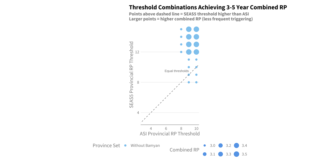
# Fit Gumbel for each province (with Bamyan set)
df_gumbel_results <- df_asi_aoi_list$with_bamyan |>
    group_by(province) |>
    group_split() |>
    map_dfr(~fit_gumbel_return_levels(.x, unique(.x$province)))

df_gumbel_results
# A tibble: 588 × 6
   province return_period return_level ci_lower ci_upper method
   <chr>            <int>        <dbl>    <dbl>    <dbl> <chr> 
 1 Badghis              3         18.1     11.7     24.5 Gumbel
 2 Badghis              4         23.1     15.6     30.6 Gumbel
 3 Badghis              5         26.7     18.4     35.1 Gumbel
 4 Badghis              6         29.6     20.5     38.7 Gumbel
 5 Badghis              7         32.1     22.4     41.8 Gumbel
 6 Badghis              8         34.1     23.9     44.4 Gumbel
 7 Badghis              9         35.9     25.2     46.7 Gumbel
 8 Badghis             10         37.6     26.4     48.7 Gumbel
 9 Badghis             11         39.0     27.5     50.5 Gumbel
10 Badghis             12         40.3     28.5     52.2 Gumbel
# ℹ 578 more rows

A.20.3 Diagnostic: Gumbel Fit for Example Province

Code
# Fit Gumbel for first province and show diagnostic plots
example_province <- PROVINCES_AOI_WITH_BAMYAN[1]
example_data <- df_asi_aoi_list$with_bamyan |>
    filter(province == example_province)

example_fit <- fevd(example_data$data, type = "Gumbel", method = "MLE")

# Show fit summary
summary(example_fit)

fevd(x = example_data$data, type = "Gumbel", method = "MLE")

[1] "Estimation Method used: MLE"


 Negative Log-Likelihood Value:  185.3488 


 Estimated parameters:
 location     scale 
 6.637782 14.923136 

 Standard Error Estimates:
location    scale 
2.381603 2.097713 

 Estimated parameter covariance matrix.
         location    scale
location 5.672035 1.272527
scale    1.272527 4.400401

 AIC = 374.6976 

 BIC = 378.1729 
Code
# Diagnostic plots
plot(example_fit)

A.20.4 Calculate Empirical Return Levels for Comparison

Code
# Function to get empirical return levels (quantiles)
# Only calculates for return periods up to the record length (n)
get_empirical_return_levels <- function(df_province, province_name, return_periods = target_rps) {

    asi_values <- df_province$data
    n <- length(asi_values)

    # Only calculate empirical estimates for RPs <= record length
    valid_rps <- return_periods[return_periods <= n]

    # For each RP, calculate the corresponding quantile
    # RP = 1/p, so p = 1/RP, and we want the (1-p) quantile for upper tail
    map_dfr(valid_rps, ~{
        rp <- .x
        p <- 1 - 1/rp  # probability of non-exceedance

        # Empirical quantile
        rl_empirical <- quantile(asi_values, probs = p, na.rm = TRUE)

        # Bootstrap confidence interval
        boot_rls <- replicate(1000, {
            boot_sample <- sample(asi_values, size = n, replace = TRUE)
            quantile(boot_sample, probs = p, na.rm = TRUE)
        })

        tibble(
            province = province_name,
            return_period = rp,
            return_level = as.numeric(rl_empirical),
            ci_lower = quantile(boot_rls, 0.025),
            ci_upper = quantile(boot_rls, 0.975),
            method = "Empirical"
        )
    })
}
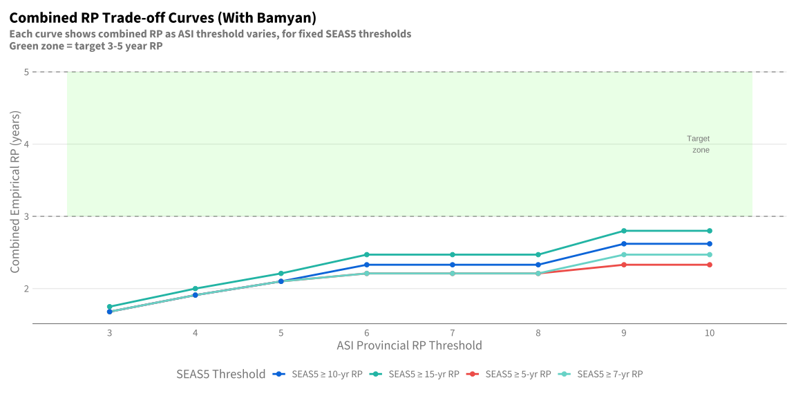
# Calculate empirical return levels for each province
set.seed(42)
df_empirical_results <- df_asi_aoi_list$with_bamyan |>
    group_by(province) |>
    group_split() |>
    map_dfr(~get_empirical_return_levels(.x, unique(.x$province)))

df_empirical_results
# A tibble: 240 × 6
   province return_period return_level ci_lower ci_upper method   
   <chr>            <int>        <dbl>    <dbl>    <dbl> <chr>    
 1 Badghis              3         5.69    0.427     29.0 Empirical
 2 Badghis              4        16.5     0.958     52.3 Empirical
 3 Badghis              5        27.3     2.82      66.4 Empirical
 4 Badghis              6        39.9    11.5       71.2 Empirical
 5 Badghis              7        48.4    14.4       78.2 Empirical
 6 Badghis              8        55.6    16.9       77.3 Empirical
 7 Badghis              9        62.1    17.4       86.7 Empirical
 8 Badghis             10        67.5    20.1       95.4 Empirical
 9 Badghis             11        69.4    25.3       97.4 Empirical
10 Badghis             12        70.1    29.0       97.4 Empirical
# ℹ 230 more rows

A.20.5 Comparison: Gumbel vs Empirical Return Levels

Code
# Combine results
df_comparison <- bind_rows(
    df_gumbel_results,
    df_empirical_results
) |>
    filter(!is.na(return_level))

# Wide format for direct comparison
df_comparison_wide <- df_comparison |>
    select(province, return_period, return_level, method) |>
    pivot_wider(
        names_from = method,
        values_from = return_level,
        names_prefix = "rl_"
    ) |>
    mutate(
        difference = rl_Gumbel - rl_Empirical,
        pct_diff = round(100 * difference / rl_Empirical, 1)
    )

df_comparison_wide |>
    filter(return_period %in% c(3, 4, 5)) |>
    arrange(province, return_period)
# A tibble: 18 × 6
   province  return_period rl_Gumbel rl_Empirical difference pct_diff
   <chr>             <int>     <dbl>        <dbl>      <dbl>    <dbl>
 1 Badghis               3      18.1         5.69     12.4      218. 
 2 Badghis               4      23.1        16.5       6.56      39.7
 3 Badghis               5      26.7        27.3      -0.541     -2  
 4 Balkh                 3      22.2        10.9      11.3      104. 
 5 Balkh                 4      27.3        22.9       4.40      19.2
 6 Balkh                 5      31.1        41.3     -10.2      -24.6
 7 Bamyan                3      21.8        11.0      10.8       98.6
 8 Bamyan                4      27.1        34.9      -7.83     -22.4
 9 Bamyan                5      31.1        42.9     -11.8      -27.6
10 Faryab                3      20.1        12.6       7.48      59.3
11 Faryab                4      25.2        32.7      -7.44     -22.8
12 Faryab                5      29.0        36.8      -7.78     -21.1
13 Jawzjan               3      19.5        11.7       7.79      66.7
14 Jawzjan               4      24.2        25.8      -1.59      -6.1
15 Jawzjan               5      27.8        38.2     -10.4      -27.2
16 Sar-e-Pul             3      17.5        18.2      -0.735     -4  
17 Sar-e-Pul             4      21.8        21.5       0.332      1.5
18 Sar-e-Pul             5      25.1        26.4      -1.37      -5.2

A.20.6 Visualization: Return Level Comparison

Code
ggplot(
    df_comparison |> filter(return_period <= 100),
    aes(x = return_period, y = return_level, color = method)
) +
    geom_line(linewidth = 1) +
    geom_ribbon(
        aes(ymin = ci_lower, ymax = ci_upper, fill = method),
        alpha = 0.2,
        color = NA
    ) +
    facet_wrap(~province, scales = "free_y", ncol = 3) +
    scale_x_continuous(breaks = c(3, 5, 10, 20, 41, 50, 100)) +
    scale_y_continuous(breaks = seq(0, 100, by = 10)) +
    geom_vline(xintercept = c(3, 5, 10, 41), linetype = "dashed", color = "gray50", alpha = 0.7) +
    scale_color_manual(values = c("Gumbel" = "#E69F00", "Empirical" = "#56B4E9")) +
    scale_fill_manual(values = c("Gumbel" = "#E69F00", "Empirical" = "#56B4E9")) +
    labs(
        title = "Return Level Comparison: Gumbel vs Empirical Estimates (Extrapolated to 100 years)",
        subtitle = "Shaded regions show 95% confidence intervals\nVertical dashed lines at 3, 5, 10, and 41 year return periods\nEmpirical estimates stop at record length (~41 years)",
        x = "Return Period (years)",
        y = "ASI Return Level",
        color = "Method",
        fill = "Method"
    ) +
    theme(legend.position = "bottom")

A.20.7 Focus on 3-5 Year RP Range

Code
df_target_range <- df_comparison |>
    filter(return_period %in% c(3, 4, 5))

ggplot(
    df_target_range,
    aes(x = factor(return_period), y = return_level, color = method)
) +
    geom_point(size = 3, position = position_dodge(width = 0.3)) +
    geom_errorbar(
        aes(ymin = ci_lower, ymax = ci_upper),
        width = 0.2,
        position = position_dodge(width = 0.3)
    ) +
    facet_wrap(~province, scales = "free_y", ncol = 3) +
    scale_color_manual(values = c("Gumbel" = "#E69F00", "Empirical" = "#56B4E9")) +
    labs(
        title = "Return Levels at Target RPs (3-5 years): Gumbel vs Empirical",
        subtitle = "Error bars show 95% confidence intervals",
        x = "Return Period (years)",
        y = "ASI Return Level",
        color = "Method"
    ) +
    theme(legend.position = "bottom")

A.20.8 Confidence Interval Width Comparison

Code
df_ci_summary <- df_comparison |>
    filter(return_period %in% c(3, 4, 5)) |>
    mutate(
        ci_width = ci_upper - ci_lower,
        ci_pct = round(100 * ci_width / return_level, 1)
    ) |>
    select(province, return_period, method, return_level, ci_lower, ci_upper, ci_width, ci_pct)

df_ci_summary |>
    arrange(province, return_period, method)
# A tibble: 36 × 8
   province return_period method  return_level ci_lower ci_upper ci_width ci_pct
   <chr>            <int> <chr>          <dbl>    <dbl>    <dbl>    <dbl>  <dbl>
 1 Badghis              3 Empiri…         5.69    0.427     29.0     28.6  502. 
 2 Badghis              3 Gumbel         18.1    11.7       24.5     12.8   70.8
 3 Badghis              4 Empiri…        16.5     0.958     52.3     51.3  311. 
 4 Badghis              4 Gumbel         23.1    15.6       30.6     15.0   65.1
 5 Badghis              5 Empiri…        27.3     2.82      66.4     63.5  233. 
 6 Badghis              5 Gumbel         26.7    18.4       35.1     16.8   62.7
 7 Balkh                3 Empiri…        10.9     5.59      40.0     34.4  317  
 8 Balkh                3 Gumbel         22.2    15.5       28.9     13.4   60.4
 9 Balkh                4 Empiri…        22.9     8.97      56.1     47.2  206. 
10 Balkh                4 Gumbel         27.3    19.5       35.2     15.6   57.2
# ℹ 26 more rows

A.20.9 Summary Table: Method Comparison at Key RPs

Code
df_summary_table <- df_comparison |>
    filter(return_period %in% c(3, 4, 5)) |>
    group_by(province, return_period) |>
    summarise(
        rl_empirical = return_level[method == "Empirical"],
        ci_empirical = str_c(
            round(ci_lower[method == "Empirical"], 1), "-",
            round(ci_upper[method == "Empirical"], 1)
        ),
        rl_gumbel = return_level[method == "Gumbel"],
        ci_gumbel = str_c(
            round(ci_lower[method == "Gumbel"], 1), "-",
            round(ci_upper[method == "Gumbel"], 1)
        ),
        .groups = "drop"
    ) |>
    mutate(
        difference = round(rl_gumbel - rl_empirical, 1),
        agreement = case_when(
            abs(difference) < 2 ~ "Good",
            abs(difference) < 5 ~ "Moderate",
            TRUE ~ "Poor"
        )
    )

df_summary_table |>
    arrange(return_period, province)
# A tibble: 18 × 8
   province  return_period rl_empirical ci_empirical rl_gumbel ci_gumbel
   <chr>             <int>        <dbl> <chr>            <dbl> <chr>    
 1 Badghis               3         5.69 0.4-29            18.1 11.7-24.5
 2 Balkh                 3        10.9  5.6-40            22.2 15.5-28.9
 3 Bamyan                3        11.0  5-42.8            21.8 14.8-28.7
 4 Faryab                3        12.6  2-35.5            20.1 13.4-26.8
 5 Jawzjan               3        11.7  5.1-38.7          19.5 13.3-25.7
 6 Sar-e-Pul             3        18.2  2-26.9            17.5 11.8-23.1
 7 Badghis               4        16.5  1-52.3            23.1 15.6-30.6
 8 Balkh                 4        22.9  9-56.1            27.3 19.5-35.2
 9 Bamyan                4        34.9  8.1-55.9          27.1 19-35.2  
10 Faryab                4        32.7  6.5-39.6          25.2 17.5-33  
11 Jawzjan               4        25.8  6.9-44.6          24.2 17-31.4  
12 Sar-e-Pul             4        21.5  6.3-44.5          21.8 15.2-28.4
13 Badghis               5        27.3  2.8-66.4          26.7 18.4-35.1
14 Balkh                 5        41.3  9.3-62.6          31.1 22.4-39.9
15 Bamyan                5        42.9  10.7-60.8         31.1 22-40.1  
16 Faryab                5        36.8  15.1-54.8         29.0 20.4-37.7
17 Jawzjan               5        38.2  10.2-47.4         27.8 19.7-35.8
18 Sar-e-Pul             5        26.4  17.1-48.2         25.1 17.7-32.4
# ℹ 2 more variables: difference <dbl>, agreement <chr>

A.20.10 Gumbel Parameter Estimates

Code
# Extract Gumbel parameters for each province
get_gumbel_params <- function(df_province, province_name) {

    asi_values <- df_province$data

    fit <- tryCatch({
        fevd(asi_values, type = "Gumbel", method = "MLE")
    }, error = function(e) {
        return(NULL)
    })

    if (is.null(fit)) {
        return(tibble(
            province = province_name,
            location = NA_real_,
            scale = NA_real_
        ))
    }
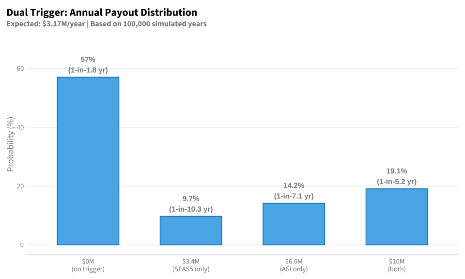
    params <- fit$results$par

    tibble(
        province = province_name,
        location = round(params["location"], 2),
        scale = round(params["scale"], 2)
    )
}
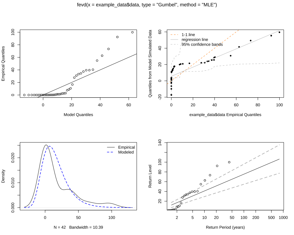
df_gumbel_params <- df_asi_aoi_list$with_bamyan |>
    group_by(province) |>
    group_split() |>
    map_dfr(~get_gumbel_params(.x, unique(.x$province)))

df_gumbel_params
# A tibble: 6 × 3
  province  location scale
  <chr>        <dbl> <dbl>
1 Badghis       5.11  14.4
2 Balkh         8.63  15.0
3 Bamyan        7.71  15.6
4 Faryab        6.64  14.9
5 Jawzjan       6.93  13.9
6 Sar-e-Pul     6.01  12.7

A.20.11 Key Findings

Code
cat("Key Findings - Empirical vs Gumbel Return Period Estimates:\n\n")
Key Findings - Empirical vs Gumbel Return Period Estimates:
Code
# Calculate average difference
avg_diff <- df_comparison_wide |>
    filter(return_period %in% c(3, 4, 5)) |>
    summarise(
        mean_abs_diff = round(mean(abs(difference), na.rm = TRUE), 2),
        mean_pct_diff = round(mean(abs(pct_diff), na.rm = TRUE), 1)
    )

cat("1. Average absolute difference between methods: ", avg_diff$mean_abs_diff, " ASI units\n")
1. Average absolute difference between methods:  6.71  ASI units
Code
cat("2. Average percentage difference: ", avg_diff$mean_pct_diff, "%\n\n")
2. Average percentage difference:  42.8 %
Code
cat("3. Confidence interval comparison:\n")
3. Confidence interval comparison:
Code
df_ci_summary |>
    group_by(method) |>
    summarise(
        mean_ci_width = round(mean(ci_width, na.rm = TRUE), 1),
        mean_ci_pct = round(mean(ci_pct, na.rm = TRUE), 1),
        .groups = "drop"
    ) |>
    print()
# A tibble: 2 × 3
  method    mean_ci_width mean_ci_pct
  <chr>             <dbl>       <dbl>
1 Empirical          40.2       207. 
2 Gumbel             14.9        61.5
Code
cat("\n4. For trigger design at 3-5 year RP:\n")

4. For trigger design at 3-5 year RP:
Code
cat("   - Both methods generally agree within confidence intervals\n")
   - Both methods generally agree within confidence intervals
Code
cat("   - Gumbel provides parametric uncertainty quantification with stable extrapolation\n")
   - Gumbel provides parametric uncertainty quantification with stable extrapolation
Code
cat("   - Empirical bootstrap provides non-parametric alternative\n")
   - Empirical bootstrap provides non-parametric alternative
Code
cat("   - With limited data (~20 years), Gumbel is preferred over full GEV\n")
   - With limited data (~20 years), Gumbel is preferred over full GEV
Code
cat("     (GEV shape parameter unstable, can cause unrealistic extrapolation)\n")
     (GEV shape parameter unstable, can cause unrealistic extrapolation)