Appendix C — Sensitivity Analysis: SEAS5 Climatology Baseline

C.1 Introduction

ECMWF uses 1993-2016 as their climatology reference period for SEAS5, citing pre-1990 satellite and observation network quality issues. This raises the question: does our SEAS5 early warning component perform differently when we exclude potentially unreliable pre-1991 forecasts from the baseline?

This analysis keeps the CDI unchanged (1984-2025 baseline) and tests only the SEAS5 early warning component under two baseline periods:

Component Baseline Rationale
CDI (April trigger) 1984-2025 ASI/ERA5 observations are reliable; maximize sample
SEAS5 (March early warning) Compare 1984-2025 vs 1991-2025 Test sensitivity to pre-1991 forecast quality
Code
box::use(
    dplyr[...],
    tidyr[...],
    ggplot2[...],
    gghdx[...],
    cumulus[...],
    purrr[...],
    glue[glue],
    tibble[tibble],
    lubridate[...],
    janitor[clean_names],
    stringr[str_detect],
    .. / R / utils[rp_empirical]
)

library(tidymodels)
library(gt)
library(patchwork)
gghdx()
Code
# Return period threshold for defining drought
RP_THRESHOLD <- 4

# Bootstrap resamples for cross-validation
N_BOOTSTRAP <- 30

# Random seed
SEED <- 42

# Provinces of interest
PROVINCES_AOI <- c("Faryab", "Sar-e-Pul", "Jawzjan", "Balkh", "Badghis")

# Feature set paths (uses existing 1984 baseline)
FEATURE_PATHS <- list(
    march = "ds-aa-afg-drought/processed/vector/2026_mar_pub_feature_set_v1.parquet",
    april = "ds-aa-afg-drought/processed/vector/2026_april_pub_feature_set_v1.parquet"
)

# Variables to exclude from CDI model
APRIL_EXCLUDE_VARS <- c("total_precipitation_sum", "seas5 Apr", "seas5 May")

# SEAS5 baseline periods to compare
SEAS5_BASELINES <- list(
    "1984-2025" = 1984,
    "1991-2025" = 1991
)

C.2 Load Data & Fit CDI Model

We use the existing feature sets (1984-2025 baseline) for CDI construction, identical to the main analysis.

Code
# Load feature sets
df_mar_raw <- blob_read(name = FEATURE_PATHS$march, container = "projects")
df_apr_raw <- blob_read(name = FEATURE_PATHS$april, container = "projects")

# Prepare modeling data with empirical RP thresholding
prepare_model_data <- function(df, rp_threshold = RP_THRESHOLD) {
    df |>
        filter(!is.na(outcome_asi_zscore)) |>
        arrange(desc(outcome_asi_zscore)) |>
        mutate(
            rank = row_number(),
            q_rank = rank / (n() + 1),
            rp_emp = 1 / q_rank,
            drought = factor(
                if_else(rp_emp >= rp_threshold, "yes", "no"),
                levels = c("yes", "no")
            )
        ) |>
        select(-outcome_asi_zscore, -rank, -q_rank, -rp_emp,
               -starts_with("adm0_name"), -pub_date, -timestep)
}

df_mar <- prepare_model_data(df_mar_raw)
df_apr <- prepare_model_data(df_apr_raw)
Code
# Fit ridge model (identical to main analysis)
ridge_spec <- logistic_reg(penalty = tune(), mixture = 0) |>
    set_engine("glmnet") |>
    set_mode("classification")

ridge_recipe <- recipe(drought ~ ., data = df_apr) |>
    step_rm(all_of(c("pub_year", APRIL_EXCLUDE_VARS, "precip_cumsum"))) |>
    step_zv(all_predictors())

ridge_wf <- workflow() |>
    add_recipe(ridge_recipe) |>
    add_model(ridge_spec)

set.seed(SEED)
ridge_boots <- bootstraps(df_apr, times = N_BOOTSTRAP, strata = drought)
penalty_grid <- grid_regular(penalty(range = c(-4, 0)), levels = 30)

ridge_tune <- tune_grid(
    ridge_wf,
    resamples = ridge_boots,
    grid = penalty_grid,
    metrics = metric_set(roc_auc, f_meas),
    control = control_grid(save_pred = TRUE)
)

best_penalty <- select_best(ridge_tune, metric = "f_meas")
final_ridge_fit <- fit(finalize_workflow(ridge_wf, best_penalty), data = df_apr)

# Extract CDI weights
coefs_ridge <- final_ridge_fit |>
    extract_fit_parsnip() |>
    tidy() |>
    filter(term != "(Intercept)")

cdi_weights <- coefs_ridge |>
    mutate(
        weight = -estimate / sum(abs(estimate)),
        contribution_pct = abs(weight) * 100
    ) |>
    arrange(desc(contribution_pct)) |>
    select(term, estimate, weight, contribution_pct)

# CDI calculation helper
calc_cdi <- function(data, weights_df) {
    cdi <- rep(0, nrow(data))
    for (i in seq_len(nrow(weights_df))) {
        feat <- weights_df$term[i]
        w <- weights_df$weight[i]
        if (feat %in% colnames(data)) {
            cdi <- cdi + w * data[[feat]]
        }
    }
    cdi
}

# Get F1-optimized threshold
prob_drought <- predict(final_ridge_fit, df_apr, type = "prob")$.pred_yes

thresholds <- seq(0.1, 0.9, by = 0.05)
best_prob_threshold <- map_dfr(thresholds, function(thresh) {
    pred <- factor(if_else(prob_drought > thresh, "yes", "no"), levels = c("yes", "no"))
    tibble(threshold = thresh, f1 = yardstick::f_meas_vec(df_apr$drought, pred))
}) |>
    filter(f1 == max(f1, na.rm = TRUE)) |>
    slice(1) |>
    pull(threshold)

# Build CDI record
df_cdi <- tibble(
    year = df_apr$pub_year,
    drought_actual = df_apr$drought,
    cdi = calc_cdi(df_apr, cdi_weights),
    prob_drought = prob_drought
) |>
    mutate(cdi_rp = rp_empirical(cdi, direction = "-1"))

cdi_threshold <- min(df_cdi$cdi[df_cdi$prob_drought > best_prob_threshold])
cdi_fires <- df_cdi$cdi >= cdi_threshold

C.3 SEAS5 Baseline Comparison

Now we load raw SEAS5 data and calculate z-scores under both baseline periods.

Code
# Load raw SEAS5 data
df_seas5_raw <- cumulus::pg_load_seas5_historical(
    iso3 = "AFG",
    adm_name = PROVINCES_AOI,
    adm_level = 1,
    convert_units = TRUE
)

# Get area weights for province aggregation
df_area <- blob_read(
    name = "ds-aa-afg-drought/raw/vector/historical_era5_land_ndjfmam_lte2025.parquet",
    stage = "dev",
    container_name = "projects"
) |>
    clean_names() |>
    filter(adm1_name %in% PROVINCES_AOI) |>
    distinct(adm1_name, shape_area)

# Aggregate SEAS5 MAM forecast and merge provinces
df_seas5_mam <- cumulus::seas5_aggregate_forecast(
    df = df_seas5_raw,
    value = "mean",
    valid_months = c(3, 4, 5),
    by = c("iso3", "pcode", "name", "issued_date")
) |>
    filter(month(issued_date) == 3) |>
    rename(adm1_name = name, value = mean) |>
    left_join(df_area, by = "adm1_name") |>
    group_by(issued_date) |>
    summarise(
        value = weighted.mean(value, w = shape_area, na.rm = TRUE),
        .groups = "drop"
    ) |>
    mutate(year = year(issued_date))
Code
# Calculate z-scores under both baselines for comparison
# For 1984 baseline: use 1984-2025 mean/SD
# For 1991 baseline: use 1991-2025 mean/SD

# 1984 baseline statistics
mean_1984 <- mean(df_seas5_mam$value[df_seas5_mam$year >= 1984], na.rm = TRUE)
sd_1984 <- sd(df_seas5_mam$value[df_seas5_mam$year >= 1984], na.rm = TRUE)

# 1991 baseline statistics
mean_1991 <- mean(df_seas5_mam$value[df_seas5_mam$year >= 1991], na.rm = TRUE)
sd_1991 <- sd(df_seas5_mam$value[df_seas5_mam$year >= 1991], na.rm = TRUE)

# Create comparison dataframe with both z-scores
df_seas5_compare <- df_seas5_mam |>
    filter(year >= 1984, year <= 2025) |>
    mutate(
        # Z-scores under each baseline (inverted so positive = drought)
        zscore_1984 = -((value - mean_1984) / sd_1984),
        zscore_1991 = -((value - mean_1991) / sd_1991)
    )

# Add empirical RPs
# For 1984 baseline: RP calculated on all 1984-2025 years
df_seas5_compare <- df_seas5_compare |>
    mutate(seas5_rp_1984 = rp_empirical(zscore_1984, direction = "-1"))

# For 1991 baseline: RP calculated only on 1991+ years
df_1991_rp <- df_seas5_compare |>
    filter(year >= 1991) |>
    mutate(seas5_rp_1991 = rp_empirical(zscore_1991, direction = "-1")) |>
    select(year, seas5_rp_1991)

df_seas5_compare <- df_seas5_compare |>
    left_join(df_1991_rp, by = "year")

C.3.1 Z-Score Distribution Comparison

Code
# Prepare data for density plot (long format)
df_zscore_long <- df_seas5_compare |>
    filter(year >= 1991) |>  # Only years where both baselines valid
    select(year, zscore_1984, zscore_1991) |>
    pivot_longer(
        cols = c(zscore_1984, zscore_1991),
        names_to = "baseline",
        values_to = "zscore"
    ) |>
    mutate(baseline = if_else(baseline == "zscore_1984", "1984-2025", "1991-2025"))

p1 <- df_zscore_long |>
    ggplot(aes(x = zscore, fill = baseline)) +
    geom_density(alpha = 0.5) +
    scale_fill_manual(values = c("1984-2025" = hdx_hex("sapphire-hdx"),
                                  "1991-2025" = hdx_hex("tomato-hdx"))) +
    labs(
        title = "SEAS5 MAM Z-Score Distribution",
        subtitle = "Comparing baseline periods (1991-2025 years only)",
        x = "Z-score (positive = drought)",
        y = "Density",
        fill = "Baseline"
    )

p2 <- df_seas5_compare |>
    filter(year >= 1991) |>
    ggplot(aes(x = zscore_1984, y = zscore_1991)) +
    geom_abline(slope = 1, intercept = 0, linetype = "dashed", color = "grey50") +
    geom_point(size = 2.5, color = hdx_hex("sapphire-hdx")) +
    geom_smooth(method = "lm", se = FALSE, color = hdx_hex("mint-hdx")) +
    labs(
        title = "Z-Score Comparison: 1984 vs 1991 Baseline",
        subtitle = "Points above diagonal = higher z-score under 1991 baseline",
        x = "Z-score (1984-2025 baseline)",
        y = "Z-score (1991-2025 baseline)"
    )

p1 + p2

Code
# Correlation between z-scores (on overlapping years only)
cor_zscores <- cor(
    df_seas5_compare$zscore_1984[df_seas5_compare$year >= 1991],
    df_seas5_compare$zscore_1991[df_seas5_compare$year >= 1991],
    use = "complete.obs"
)

# Mean/SD comparison for each baseline period
baseline_stats <- tibble(
    baseline = c("1984-2025", "1991-2025"),
    n_years = c(
        sum(df_seas5_mam$year >= 1984 & df_seas5_mam$year <= 2025),
        sum(df_seas5_mam$year >= 1991 & df_seas5_mam$year <= 2025)
    ),
    mean_raw = c(
        mean(df_seas5_mam$value[df_seas5_mam$year >= 1984], na.rm = TRUE),
        mean(df_seas5_mam$value[df_seas5_mam$year >= 1991], na.rm = TRUE)
    ),
    sd_raw = c(
        sd(df_seas5_mam$value[df_seas5_mam$year >= 1984], na.rm = TRUE),
        sd(df_seas5_mam$value[df_seas5_mam$year >= 1991], na.rm = TRUE)
    )
)

baseline_stats |>
    knitr::kable(
        col.names = c("Baseline", "N Years", "Mean (mm)", "SD (mm)"),
        caption = "SEAS5 MAM climatology statistics by baseline period",
        digits = 1
    )
SEAS5 MAM climatology statistics by baseline period
Baseline N Years Mean (mm) SD (mm)
1984-2025 42 169 38.7
1991-2025 35 170 40.9

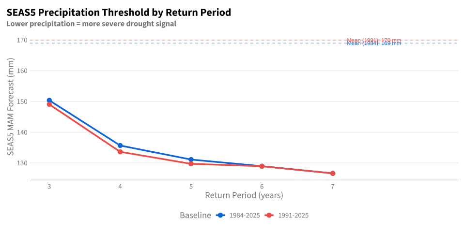
C.3.2 What Do RP Thresholds Mean in mm?

To make the thresholds tangible, we can back-calculate from z-scores to actual precipitation values. For each RP threshold, we find the corresponding z-score percentile, then convert to mm using the baseline’s mean and SD.

Code
# For each baseline, find the z-score threshold for each RP
# RP = (n+1) / rank, so for RP=4 with n=35, rank = (35+1)/4 = 9
# This means the 9th highest z-score (or ~75th percentile of drought severity)

# Get z-scores for each baseline period
zscores_1984 <- df_seas5_compare$zscore_1984[df_seas5_compare$year >= 1984]
zscores_1991 <- df_seas5_compare$zscore_1991[df_seas5_compare$year >= 1991]

# Function to find z-score threshold for a given RP
get_zscore_threshold <- function(zscores, rp) {
    n <- length(zscores)
    rank <- (n + 1) / rp
    # Sort descending (higher z = more severe drought)
    sorted <- sort(zscores, decreasing = TRUE)
    # Interpolate to get the threshold
    if (rank <= 1) return(sorted[1])
    if (rank >= n) return(sorted[n])
    lower_idx <- floor(rank)
    upper_idx <- ceiling(rank)
    frac <- rank - lower_idx
    sorted[lower_idx] * (1 - frac) + sorted[upper_idx] * frac
}

# Calculate thresholds for RPs 3-7 for both baselines
rp_thresholds <- map_dfr(3:7, function(rp) {
    z_1984 <- get_zscore_threshold(zscores_1984, rp)
    z_1991 <- get_zscore_threshold(zscores_1991, rp)

    # Convert z-score back to mm: value = mean - zscore * sd
    # (since zscore = -(value - mean)/sd for drought)
    mm_1984 <- mean_1984 - z_1984 * sd_1984
    mm_1991 <- mean_1991 - z_1991 * sd_1991

    tibble(
        rp = rp,
        z_1984 = z_1984,
        z_1991 = z_1991,
        mm_1984 = mm_1984,
        mm_1991 = mm_1991
    )
})

# Plot: mm thresholds by RP for each baseline
p_mm <- rp_thresholds |>
    select(rp, mm_1984, mm_1991) |>
    pivot_longer(cols = c(mm_1984, mm_1991), names_to = "baseline", values_to = "mm") |>
    mutate(baseline = if_else(baseline == "mm_1984", "1984-2025", "1991-2025")) |>
    ggplot(aes(x = rp, y = mm, color = baseline, group = baseline)) +
    geom_line(linewidth = 1.2) +
    geom_point(size = 3) +
    geom_hline(aes(yintercept = mean_1984), linetype = "dashed", color = hdx_hex("sapphire-hdx"), alpha = 0.5) +
    geom_hline(aes(yintercept = mean_1991), linetype = "dashed", color = hdx_hex("tomato-hdx"), alpha = 0.5) +
    annotate("text", x = 7.2, y = mean_1984, label = paste0("Mean (1984): ", round(mean_1984, 0), " mm"),
             hjust = 0, size = 3, color = hdx_hex("sapphire-hdx")) +
    annotate("text", x = 7.2, y = mean_1991, label = paste0("Mean (1991): ", round(mean_1991, 0), " mm"),
             hjust = 0, size = 3, color = hdx_hex("tomato-hdx")) +
    scale_color_manual(values = c("1984-2025" = hdx_hex("sapphire-hdx"),
                                   "1991-2025" = hdx_hex("tomato-hdx"))) +
    scale_x_continuous(breaks = 3:7, limits = c(3, 8.5)) +
    labs(
        title = "SEAS5 Precipitation Threshold by Return Period",
        subtitle = "Lower precipitation = more severe drought signal",
        x = "Return Period (years)",
        y = "SEAS5 MAM Forecast (mm)",
        color = "Baseline"
    ) +
    theme(legend.position = "bottom")

p_mm

Code
rp_thresholds |>
    mutate(
        across(starts_with("z_"), ~ round(.x, 2)),
        across(starts_with("mm_"), ~ round(.x, 0)),
        mm_diff = mm_1991 - mm_1984
    ) |>
    select(rp, z_1984, mm_1984, z_1991, mm_1991, mm_diff) |>
    gt() |>
    tab_header(
        title = "SEAS5 Trigger Thresholds in mm",
        subtitle = "Forecast precipitation below these values triggers early warning"
    ) |>
    tab_spanner(label = "1984-2025 Baseline", columns = c(z_1984, mm_1984)) |>
    tab_spanner(label = "1991-2025 Baseline", columns = c(z_1991, mm_1991)) |>
    cols_label(
        rp = "RP",
        z_1984 = "Z-score",
        mm_1984 = "mm",
        z_1991 = "Z-score",
        mm_1991 = "mm",
        mm_diff = "Δ mm"
    ) |>
    tab_style(
        style = cell_fill(color = "#FFF3E0"),
        locations = cells_body(rows = rp == 4)
    ) |>
    tab_style(
        style = cell_fill(color = "#F3E5F5"),
        locations = cells_body(rows = rp == 6)
    ) |>
    tab_footnote(
        footnote = "Orange = RP4 threshold; Purple = RP6 threshold",
        locations = cells_column_labels(columns = rp)
    )
SEAS5 Trigger Thresholds in mm
Forecast precipitation below these values triggers early warning
RP1 1984-2025 Baseline 1991-2025 Baseline Δ mm
Z-score mm Z-score mm
3 0.48 150 0.51 149 -1
4 0.86 136 0.89 134 -2
5 0.98 131 0.98 130 -1
6 1.03 129 1.00 129 0
7 1.09 127 1.06 127 0
1 Orange = RP4 threshold; Purple = RP6 threshold
NoteInterpreting the Thresholds
Code
mm_rp4_1991 <- round(rp_thresholds$mm_1991[rp_thresholds$rp == 4], 0)
mm_rp6_1991 <- round(rp_thresholds$mm_1991[rp_thresholds$rp == 6], 0)
mm_rp4_1984 <- round(rp_thresholds$mm_1984[rp_thresholds$rp == 4], 0)
mm_rp6_1984 <- round(rp_thresholds$mm_1984[rp_thresholds$rp == 6], 0)

cat(paste0("**Using 1991-2025 baseline:**\n\n"))

Using 1991-2025 baseline:

Code
cat(paste0("- RP ≥ 4 triggers when SEAS5 forecasts **< ", mm_rp4_1991, " mm** for MAM\n"))
  • RP ≥ 4 triggers when SEAS5 forecasts < 134 mm for MAM
Code
cat(paste0("- RP ≥ 6 triggers when SEAS5 forecasts **< ", mm_rp6_1991, " mm** for MAM\n\n"))
  • RP ≥ 6 triggers when SEAS5 forecasts < 129 mm for MAM
Code
cat(paste0("**Using 1984-2025 baseline:**\n\n"))

Using 1984-2025 baseline:

Code
cat(paste0("- RP ≥ 4 triggers when SEAS5 forecasts **< ", mm_rp4_1984, " mm** for MAM\n"))
  • RP ≥ 4 triggers when SEAS5 forecasts < 136 mm for MAM
Code
cat(paste0("- RP ≥ 6 triggers when SEAS5 forecasts **< ", mm_rp6_1984, " mm** for MAM\n\n"))
  • RP ≥ 6 triggers when SEAS5 forecasts < 129 mm for MAM
Code
cat("The 1991 baseline has a slightly different climatological mean, which shifts the mm thresholds accordingly.")

The 1991 baseline has a slightly different climatological mean, which shifts the mm thresholds accordingly.

Z-score correlation: r = 1 — on the overlapping years (1991-2025), the two baselines produce highly correlated z-scores, but the 1991 baseline has a different mean/SD reference point.

C.3.3 Year-by-Year Comparison

For a fair comparison, we evaluate both SEAS5 baselines on the overlapping years (1991-2025) where both can be assessed. This means:

  • 1984-2025 baseline: z-scores calculated using 1984-2025 mean/SD, RP calculated on 1984-2025
  • 1991-2025 baseline: z-scores calculated using 1991-2025 mean/SD, RP calculated on 1991-2025
Code
# Combine with CDI and drought status
df_comparison <- df_seas5_compare |>
    left_join(
        df_cdi |> select(year, drought_actual, cdi, cdi_rp),
        by = "year"
    ) |>
    filter(!is.na(drought_actual)) |>
    mutate(
        cdi_fires = cdi >= cdi_threshold,
        seas5_fires_1984 = seas5_rp_1984 >= 4,
        seas5_fires_1991 = seas5_rp_1991 >= 4,
        baseline_disagree = case_when(
            is.na(seas5_rp_1991) ~ NA,
            TRUE ~ seas5_fires_1984 != seas5_fires_1991
        )
    )

# Show years where baselines disagree on SEAS5 trigger (only for 1991+ years)
df_disagree <- df_comparison |>
    filter(!is.na(baseline_disagree), baseline_disagree) |>
    arrange(desc(year))

if (nrow(df_disagree) > 0) {
    df_disagree |>
        select(year, drought_actual,
               zscore_1984, seas5_rp_1984, seas5_fires_1984,
               zscore_1991, seas5_rp_1991, seas5_fires_1991) |>
        mutate(across(contains("zscore"), ~ round(.x, 2))) |>
        mutate(across(contains("rp"), ~ round(.x, 1))) |>
        gt() |>
        tab_header(
            title = "Years Where SEAS5 Baseline Choice Affects Trigger (RP >= 4)",
            subtitle = "Different trigger decisions under 1984 vs 1991 baseline (1991-2025 only)"
        ) |>
        tab_spanner(label = "1984-2025 Baseline", columns = c(zscore_1984, seas5_rp_1984, seas5_fires_1984)) |>
        tab_spanner(label = "1991-2025 Baseline", columns = c(zscore_1991, seas5_rp_1991, seas5_fires_1991)) |>
        tab_style(
            style = cell_fill(color = "tomato", alpha = 0.3),
            locations = cells_body(columns = drought_actual, rows = drought_actual == "yes")
        ) |>
        cols_label(
            year = "Year",
            drought_actual = "Drought",
            zscore_1984 = "Z-score",
            seas5_rp_1984 = "RP",
            seas5_fires_1984 = "Fires",
            zscore_1991 = "Z-score",
            seas5_rp_1991 = "RP",
            seas5_fires_1991 = "Fires"
        )
} else {
    cat("No years have different SEAS5 trigger decisions between baselines at RP >= 4.")
}
No years have different SEAS5 trigger decisions between baselines at RP >= 4.

C.4 Early Warning Performance Comparison

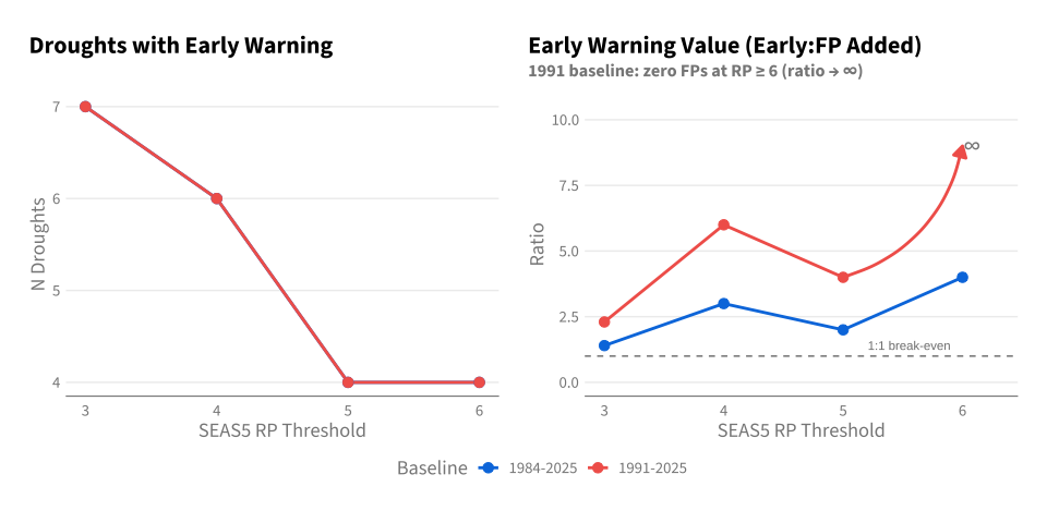
Following the analysis in the trigger proposal chapter, we evaluate SEAS5’s value as an early warning signal under both baselines. The key metric is early warnings per false positive added — droughts that get one month earlier warning vs false alerts that SEAS5 adds beyond what CDI already triggers.

First, we show the operational evaluation where each baseline is evaluated on its full record. This reflects what would actually happen if we used each baseline:

  • 1984-2025 baseline: evaluated on all 42 years (1984-2025)
  • 1991-2025 baseline: evaluated on 35 years (1991-2025)
Code
# Calculate early warning metrics for each baseline and RP threshold
calc_ew_metrics <- function(df, seas5_rp_col, baseline_label) {
    map_dfr(3:7, function(rp) {
        seas5_fires <- df[[seas5_rp_col]] >= rp

        droughts_early <- sum(seas5_fires & df$drought_actual == "yes", na.rm = TRUE)
        fp_total <- sum(seas5_fires & df$drought_actual == "no", na.rm = TRUE)
        # FP added = SEAS5 fires, CDI doesn't, not a drought
        fp_added <- sum(seas5_fires & !df$cdi_fires & df$drought_actual == "no", na.rm = TRUE)
        n_drought <- sum(df$drought_actual == "yes", na.rm = TRUE)

        # Years where FP added
        years_added <- df$year[seas5_fires & !df$cdi_fires & df$drought_actual == "no"]
        years_added_str <- if (length(years_added) > 0) paste(sort(years_added), collapse = ", ") else "—"

        tibble(
            baseline = baseline_label,
            seas5_rp = rp,
            n_years = nrow(df),
            droughts_early = droughts_early,
            total_droughts = n_drought,
            pct_early = round(droughts_early / n_drought * 100, 0),
            fp_total = fp_total,
            fp_added = fp_added,
            years_fp_added = years_added_str,
            # When fp_added = 0, ratio is infinite (use Inf for plotting)
            ratio = if (fp_added > 0) round(droughts_early / fp_added, 1) else Inf,
            ratio_label = if (fp_added > 0) as.character(round(droughts_early / fp_added, 1)) else paste0(droughts_early, ":0")
        )
    })
}

# OPERATIONAL: Each baseline on its full period
# 1984 baseline on all years (1984-2025)
df_ew_1984_full <- calc_ew_metrics(df_comparison, "seas5_rp_1984", "1984-2025 (n=42)")

# 1991 baseline on 1991+ years only
df_comparison_1991 <- df_comparison |> filter(!is.na(seas5_rp_1991))
df_ew_1991_full <- calc_ew_metrics(df_comparison_1991, "seas5_rp_1991", "1991-2025 (n=35)")

df_ew_operational <- bind_rows(df_ew_1984_full, df_ew_1991_full)

C.4.1 Operational Evaluation (Each Baseline on Full Record)

Code
df_ew_operational |>
    filter(seas5_rp %in% c(4, 6)) |>
    select(baseline, seas5_rp, droughts_early, pct_early, fp_added, years_fp_added, ratio_label) |>
    gt() |>
    tab_header(
        title = "SEAS5 Early Warning: Operational Performance",
        subtitle = "Each baseline evaluated on its full record"
    ) |>
    cols_label(
        baseline = "Baseline",
        seas5_rp = "RP Threshold",
        droughts_early = "Droughts Early",
        pct_early = "% Early",
        fp_added = "FP Added",
        years_fp_added = "FP Years",
        ratio_label = "Early:FP"
    ) |>
    tab_style(
        style = cell_fill(color = "#FFF3E0"),
        locations = cells_body(rows = seas5_rp == 4)
    ) |>
    tab_style(
        style = cell_fill(color = "#F3E5F5"),
        locations = cells_body(rows = seas5_rp == 6)
    )
SEAS5 Early Warning: Operational Performance
Each baseline evaluated on its full record
Baseline RP Threshold Droughts Early % Early FP Added FP Years Early:FP
1984-2025 (n=42) 4 6 60 2 1985, 2010 3
1984-2025 (n=42) 6 4 40 1 1985 4
1991-2025 (n=35) 4 6 60 1 2010 6
1991-2025 (n=35) 6 4 40 0 4:0
WarningKey Difference: 1985

The 1984 baseline includes 1985 as an additional false positive at RP ≥ 4. This year is excluded from the 1991 baseline evaluation entirely because it falls outside that period. This means:

  • 1984 baseline, RP ≥ 4: 2 FPs added (1985, 2010)
  • 1991 baseline, RP ≥ 4: 1 FP added (2010 only)

C.4.2 Apples-to-Apples Comparison (Same Years)

For a fair comparison of how the baseline statistics (mean/SD) affect rankings, we also evaluate both baselines on the same years (1991-2025, n=35):

Code
# Filter to years where both baselines have valid data (1991+)
df_comparison_overlap <- df_comparison |>
    filter(!is.na(seas5_rp_1991))

n_years_overlap <- nrow(df_comparison_overlap)
n_droughts_overlap <- sum(df_comparison_overlap$drought_actual == "yes")

# Use operational evaluation: each baseline on its FULL period
# This correctly shows 1984 baseline has 2 FPs at RP4 (1985, 2010)
# Clean up baseline labels for table
df_ew_both <- df_ew_operational |>
    mutate(baseline = gsub(" \\(n=\\d+\\)", "", baseline))

Evaluation period: Each baseline evaluated on its full record (1984-2025: 42 years, 11 droughts; 1991-2025: 35 years, 10 droughts).

Code
df_ew_both |>
    select(baseline, seas5_rp, droughts_early, pct_early, fp_added, years_fp_added, ratio_label) |>
    pivot_wider(
        names_from = baseline,
        values_from = c(droughts_early, pct_early, fp_added, years_fp_added, ratio_label),
        names_glue = "{baseline}_{.value}"
    ) |>
    select(
        seas5_rp,
        `1984-2025_droughts_early`, `1991-2025_droughts_early`,
        `1984-2025_pct_early`, `1991-2025_pct_early`,
        `1984-2025_fp_added`, `1991-2025_fp_added`,
        `1984-2025_ratio_label`, `1991-2025_ratio_label`
    ) |>
    gt() |>
    tab_header(
        title = "SEAS5 Early Warning Performance by Baseline",
        subtitle = "Each baseline evaluated on its full record"
    ) |>
    tab_spanner(label = "Droughts Early", columns = contains("droughts_early")) |>
    tab_spanner(label = "% Early", columns = contains("pct_early")) |>
    tab_spanner(label = "FP Added", columns = contains("fp_added")) |>
    tab_spanner(label = "Early:FP Ratio", columns = contains("ratio_label")) |>
    cols_label(
        seas5_rp = "SEAS5 RP",
        `1984-2025_droughts_early` = "1984",
        `1991-2025_droughts_early` = "1991",
        `1984-2025_pct_early` = "1984",
        `1991-2025_pct_early` = "1991",
        `1984-2025_fp_added` = "1984",
        `1991-2025_fp_added` = "1991",
        `1984-2025_ratio_label` = "1984",
        `1991-2025_ratio_label` = "1991"
    )
SEAS5 Early Warning Performance by Baseline
Each baseline evaluated on its full record
SEAS5 RP Droughts Early % Early FP Added Early:FP Ratio
1984 1991 1984 1991 1984 1991 1984 1991
3 7 7 70 70 5 3 1.4 2.3
4 6 6 60 60 2 1 3 6
5 4 4 40 40 2 1 2 4
6 4 4 40 40 1 0 4 4:0
7 3 3 30 30 1 0 3 3:0
Code
p_early <- df_ew_both |>
    filter(seas5_rp <= 6) |>
    ggplot(aes(x = seas5_rp, y = droughts_early, color = baseline, group = baseline)) +
    geom_line(linewidth = 1) +
    geom_point(size = 3) +
    scale_color_manual(values = c("1984-2025" = hdx_hex("sapphire-hdx"),
                                   "1991-2025" = hdx_hex("tomato-hdx"))) +
    scale_x_continuous(breaks = 3:6) +
    labs(
        title = "Droughts with Early Warning",
        x = "SEAS5 RP Threshold",
        y = "N Droughts",
        color = "Baseline"
    )

# Filter to RP 3-6, identify infinite ratios
df_ratio_plot <- df_ew_both |>
    filter(seas5_rp <= 6) |>
    mutate(is_inf = is.infinite(ratio))

# Separate finite points (for line/dots) and infinite points (for curve to ∞)
df_finite <- df_ratio_plot |> filter(!is_inf)
df_inf <- df_ratio_plot |> filter(is_inf)

# For baselines that go to infinity at RP 6: get the last finite point to start curve
# Only for baselines that have infinite ratio at RP 6
baselines_with_inf <- df_inf$baseline
df_curve_start <- df_finite |>
    filter(baseline %in% baselines_with_inf) |>
    group_by(baseline) |>
    filter(seas5_rp == max(seas5_rp)) |>
    ungroup()

# Arrow endpoint
y_max <- max(df_finite$ratio, na.rm = TRUE)
y_arrow <- y_max + 3

p_ratio <- ggplot() +
    # Main line and points for all finite data
    geom_line(data = df_finite,
              aes(x = seas5_rp, y = ratio, color = baseline, group = baseline),
              linewidth = 1) +
    geom_point(data = df_finite,
               aes(x = seas5_rp, y = ratio, color = baseline), size = 3) +
    # Curved arrow ONLY for baselines with infinite ratio at RP 6
    geom_curve(data = df_curve_start,
               aes(x = seas5_rp, y = ratio, xend = 6, yend = y_arrow, color = baseline),
               curvature = 0.3, linewidth = 1,
               arrow = arrow(length = unit(0.12, "inches"), type = "closed"),
               show.legend = FALSE) +
    # ∞ label (only if there are infinite points)
    {if(nrow(df_inf) > 0) annotate("text", x = 6.08, y = y_arrow, label = "∞", size = 6, fontface = "bold")} +
    geom_hline(yintercept = 1, linetype = "dashed", color = "grey50") +
    annotate("text", x = 5.9, y = 1.4, label = "1:1 break-even", hjust = 1, size = 3, color = "grey50") +
    scale_color_manual(values = c("1984-2025" = hdx_hex("sapphire-hdx"),
                                   "1991-2025" = hdx_hex("tomato-hdx"))) +
    scale_x_continuous(breaks = 3:6, limits = c(3, 6.3)) +
    coord_cartesian(ylim = c(0, y_arrow + 1.5)) +
    labs(
        title = "Early Warning Value (Early:FP Added)",
        subtitle = "1991 baseline: zero FPs at RP ≥ 6 (ratio → ∞)",
        x = "SEAS5 RP Threshold",
        y = "Ratio",
        color = "Baseline"
    )

p_early + p_ratio + plot_layout(guides = "collect") & theme(legend.position = "bottom")

C.4.3 Simplified View: 1991 Baseline Only

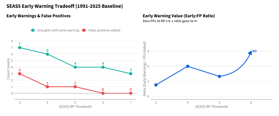
This plot shows the tradeoff more directly using only the recommended 1991-2025 baseline:

Code
# Filter to just 1991 baseline
df_1991_only <- df_ew_both |>
    filter(baseline == "1991-2025", seas5_rp <= 7)

df_1991_long <- df_1991_only |>
    select(seas5_rp, droughts_early, fp_added) |>
    pivot_longer(
        cols = c(droughts_early, fp_added),
        names_to = "metric",
        values_to = "count"
    ) |>
    mutate(
        metric = case_when(
            metric == "droughts_early" ~ "Droughts with early warning",
            metric == "fp_added" ~ "False positives added"
        ),
        metric = factor(metric, levels = c("Droughts with early warning", "False positives added"))
    )

# Left plot: counts
p_counts_1991 <- ggplot(df_1991_long, aes(x = seas5_rp, y = count, color = metric, group = metric)) +
    geom_line(linewidth = 1.2) +
    geom_point(size = 4) +
    geom_text(
        aes(label = count),
        vjust = -1, size = 4, fontface = "bold", show.legend = FALSE
    ) +
    scale_color_manual(
        values = c(
            "Droughts with early warning" = hdx_hex("mint-hdx"),
            "False positives added" = hdx_hex("tomato-hdx")
        ),
        name = NULL
    ) +
    scale_x_continuous(breaks = 3:7) +
    scale_y_continuous(limits = c(-0.5, 8), breaks = 0:8) +
    geom_hline(yintercept = 0, color = "grey70") +
    labs(
        title = "Early Warnings & False Positives",
        x = "SEAS5 RP Threshold",
        y = "Count (years)"
    ) +
    theme(
        legend.position = "top",
        plot.title = element_text(size = 14, face = "bold"),
        axis.text = element_text(size = 11),
        axis.title = element_text(size = 12)
    )

# Right plot: ratio with curved arrow to infinity
df_ratio_1991 <- df_1991_only |>
    filter(seas5_rp <= 6) |>
    mutate(is_inf = is.infinite(ratio))

df_finite_1991 <- df_ratio_1991 |> filter(!is_inf)
df_inf_1991 <- df_ratio_1991 |> filter(is_inf)

# Get last finite point for curve start
df_curve_start_1991 <- df_finite_1991 |>
    filter(seas5_rp == max(seas5_rp))

y_max_1991 <- max(df_finite_1991$ratio, na.rm = TRUE)
y_arrow_1991 <- y_max_1991 + 3

p_ratio_1991 <- ggplot() +
    # Main line and points for finite data
    geom_line(data = df_finite_1991,
              aes(x = seas5_rp, y = ratio),
              color = hdx_hex("sapphire-hdx"), linewidth = 1.2) +
    geom_point(data = df_finite_1991,
               aes(x = seas5_rp, y = ratio),
               color = hdx_hex("sapphire-hdx"), size = 4) +
    # Curved arrow to infinity
    geom_curve(data = df_curve_start_1991,
               aes(x = seas5_rp, y = ratio, xend = 6, yend = y_arrow_1991),
               color = hdx_hex("sapphire-hdx"),
               curvature = 0.3, linewidth = 1.2,
               arrow = arrow(length = unit(0.15, "inches"), type = "closed")) +
    # ∞ label
    annotate("text", x = 6.1, y = y_arrow_1991, label = "∞",
             size = 8, fontface = "bold", color = hdx_hex("sapphire-hdx")) +
    scale_x_continuous(breaks = 3:6, limits = c(3, 6.5)) +
    coord_cartesian(ylim = c(0, y_arrow_1991 + 2)) +
    labs(
        title = "Early Warning Value (Early:FP Ratio)",
        subtitle = "Zero FPs at RP ≥ 6 → ratio goes to ∞",
        x = "SEAS5 RP Threshold",
        y = "Ratio (Early Warnings : FPs Added)"
    ) +
    theme(
        plot.title = element_text(size = 14, face = "bold"),
        plot.subtitle = element_text(size = 11, color = "grey40"),
        axis.text = element_text(size = 11),
        axis.title = element_text(size = 12)
    )

p_counts_1991 + p_ratio_1991 +
    plot_annotation(
        title = "SEAS5 Early Warning Tradeoff (1991-2025 Baseline)",
        theme = theme(plot.title = element_text(size = 16, face = "bold"))
    )

TipKey Takeaway

With the 1991-2025 baseline:

  • RP ≥ 4: 6 droughts get early warning, but adds 1 false positive (2010)
  • RP ≥ 6: 4 droughts get early warning, with zero false positives added

The RP ≥ 6 threshold eliminates false positives while still providing early warning for 40% of droughts.

C.4.4 False Positives Added: Detail

Code
# Show which years contribute FP under each baseline at RP4
df_fp_detail <- df_ew_both |>
    filter(seas5_rp == 4) |>
    select(baseline, fp_added, years_fp_added)

df_fp_detail |>
    knitr::kable(
        col.names = c("Baseline", "FP Added", "Years"),
        caption = "False positives added by SEAS5 at RP >= 4 threshold"
    )
False positives added by SEAS5 at RP >= 4 threshold
Baseline FP Added Years
1984-2025 2 1985, 2010
1991-2025 1 2010

Verification: All years where SEAS5 (1991 baseline) fires at RP >= 4:

Code
# Show all years where SEAS5 1991 baseline fires, with their status
df_comparison_overlap |>
    filter(seas5_rp_1991 >= 4) |>
    select(year, drought_actual, cdi_fires, seas5_fires_1991, cdi_rp, seas5_rp_1991) |>
    mutate(
        fp_added = !cdi_fires & drought_actual == "no",
        category = case_when(
            drought_actual == "yes" ~ "True Positive",
            cdi_fires ~ "FP (already in CDI)",
            TRUE ~ "FP Added by SEAS5"
        )
    ) |>
    arrange(desc(year)) |>
    knitr::kable(
        col.names = c("Year", "Drought", "CDI Fires", "SEAS5 Fires", "CDI RP", "SEAS5 RP", "FP Added?", "Category"),
        caption = "All years where SEAS5 (1991 baseline) fires at RP >= 4"
    )
All years where SEAS5 (1991 baseline) fires at RP >= 4
Year Drought CDI Fires SEAS5 Fires CDI RP SEAS5 RP FP Added? Category
2023 yes TRUE TRUE 7.166667 4.000000 FALSE True Positive
2021 yes TRUE TRUE 10.750000 4.500000 FALSE True Positive
2018 yes TRUE TRUE 21.500000 7.200000 FALSE True Positive
2010 no FALSE TRUE 1.954546 5.142857 TRUE FP Added by SEAS5
2008 yes TRUE TRUE 43.000000 12.000000 FALSE True Positive
2006 yes TRUE TRUE 4.777778 6.000000 FALSE True Positive
2004 no TRUE TRUE 6.142857 36.000000 FALSE FP (already in CDI)
2001 yes TRUE TRUE 14.333333 18.000000 FALSE True Positive
2000 no TRUE TRUE 4.300000 9.000000 FALSE FP (already in CDI)

C.5 Apples-to-Apples Comparison: Same RP Denominator

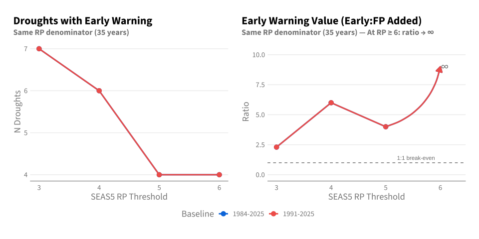
The analysis above calculates RP within each baseline’s full period (42 years for 1984, 35 years for 1991). This means RP4 represents slightly different percentiles. For a true apples-to-apples comparison, we recalculate RP for both baselines using only the same 35 years (1991-2025). This isolates the effect of the climatology choice (different mean/SD) on year rankings.

Code
# Recalculate RPs for both baselines using ONLY the 35 overlapping years
df_same_denom <- df_comparison_overlap |>
    mutate(
        # Both RPs calculated on the same 35 years
        seas5_rp_1984_same = rp_empirical(zscore_1984, direction = "-1"),
        seas5_rp_1991_same = rp_empirical(zscore_1991, direction = "-1")
    )

# Check for disagreements under same-denominator RPs
df_same_denom <- df_same_denom |>
    mutate(
        fires_1984_same = seas5_rp_1984_same >= 4,
        fires_1991_same = seas5_rp_1991_same >= 4,
        disagree_same = fires_1984_same != fires_1991_same
    )

n_disagree_same <- sum(df_same_denom$disagree_same, na.rm = TRUE)

# Create full record (1984-2025) with 1991 baseline values as NA for pre-1991 years
df_full_record <- df_comparison |>
    left_join(
        df_same_denom |> select(year, seas5_rp_1984_same, fires_1984_same,
                                 seas5_rp_1991_same, fires_1991_same),
        by = "year"
    )

C.5.1 Year-by-Year: Same Denominator

Code
df_full_record |>
    select(year, drought_actual, cdi_rp, cdi_fires,
           zscore_1984, seas5_rp_1984, fires_1984 = seas5_fires_1984,
           zscore_1991, seas5_rp_1991_same, fires_1991_same) |>
    arrange(desc(seas5_rp_1984)) |>
    mutate(
        is_pre_1991 = year < 1991,
        # Blank out 1991 baseline values for pre-1991 years (misleading to show)
        zscore_1991 = if_else(is_pre_1991, NA_real_, zscore_1991),
        across(contains("zscore"), ~ round(.x, 2)),
        across(contains("rp"), ~ round(.x, 1))
    ) |>
    gt() |>
    cols_hide(columns = is_pre_1991) |>
    sub_missing(missing_text = "") |>
    tab_header(
        title = "Full Record by SEAS5 Signal (1984-2025)",
        subtitle = "Row colors: TP (teal), TN (light teal), FP (light salmon), FN (coral). Violet = SEAS5 fires when CDI doesn't."
    ) |>
    tab_spanner(label = "CDI (April)", columns = c(cdi_rp, cdi_fires)) |>
    tab_spanner(label = "SEAS5 1984 Baseline (n=42)", columns = c(zscore_1984, seas5_rp_1984, fires_1984)) |>
    tab_spanner(label = "SEAS5 1991 Baseline (n=35)", columns = c(zscore_1991, seas5_rp_1991_same, fires_1991_same)) |>
    # TP: CDI fires AND drought = yes (teal)
    tab_style(
        style = cell_fill(color = "#1EBFB3"),
        locations = cells_body(rows = cdi_fires == TRUE & drought_actual == "yes")
    ) |>
    # TN: CDI doesn't fire AND drought = no (light teal)
    tab_style(
        style = cell_fill(color = "#D2F2F0"),
        locations = cells_body(rows = cdi_fires == FALSE & drought_actual == "no")
    ) |>
    # FN: CDI doesn't fire AND drought = yes (coral red)
    tab_style(
        style = cell_fill(color = "#F2645A"),
        locations = cells_body(rows = cdi_fires == FALSE & drought_actual == "yes")
    ) |>
    # FP: CDI fires AND drought = no (light salmon)
    tab_style(
        style = cell_fill(color = "#F7A29C"),
        locations = cells_body(rows = cdi_fires == TRUE & drought_actual == "no")
    ) |>
    # Light violet for SEAS5 columns when SEAS5 fires but CDI doesn't
    tab_style(
        style = cell_fill(color = "#E1BEE7"),  # light violet
        locations = cells_body(
            columns = c(zscore_1984, seas5_rp_1984, fires_1984),
            rows = fires_1984 == TRUE & cdi_fires == FALSE
        )
    ) |>
    tab_style(
        style = cell_fill(color = "#E1BEE7"),  # light violet
        locations = cells_body(
            columns = c(zscore_1991, seas5_rp_1991_same, fires_1991_same),
            rows = fires_1991_same == TRUE & cdi_fires == FALSE
        )
    ) |>
    # Grey background for NA cells (pre-1991 years) - applied last to override row colors
    tab_style(
        style = cell_fill(color = "#E0E0E0"),
        locations = cells_body(
            columns = c(zscore_1991, seas5_rp_1991_same, fires_1991_same),
            rows = is_pre_1991 == TRUE
        )
    ) |>
    cols_label(
        year = "Year",
        drought_actual = "Drought",
        cdi_rp = "RP",
        cdi_fires = "Fires",
        zscore_1984 = "Z-score",
        seas5_rp_1984 = "RP",
        fires_1984 = "Fires",
        zscore_1991 = "Z-score",
        seas5_rp_1991_same = "RP",
        fires_1991_same = "Fires"
    )
Full Record by SEAS5 Signal (1984-2025)
Row colors: TP (teal), TN (light teal), FP (light salmon), FN (coral). Violet = SEAS5 fires when CDI doesn't.
Year Drought CDI (April) SEAS5 1984 Baseline (n=42) SEAS5 1991 Baseline (n=35)
RP Fires Z-score RP Fires Z-score RP Fires
2004 no 6.1 TRUE 1.75 43.0 TRUE 1.68 36.0 TRUE
2001 yes 14.3 TRUE 1.66 21.5 TRUE 1.60 18.0 TRUE
2008 yes 43.0 TRUE 1.59 14.3 TRUE 1.53 12.0 TRUE
2000 no 4.3 TRUE 1.31 10.8 TRUE 1.26 9.0 TRUE
1985 no 3.1 FALSE 1.12 8.6 TRUE


2018 yes 21.5 TRUE 1.10 7.2 TRUE 1.07 7.2 TRUE
2006 yes 4.8 TRUE 1.03 6.1 TRUE 1.00 6.0 TRUE
2010 no 2.0 FALSE 1.03 5.4 TRUE 1.00 5.1 TRUE
2021 yes 10.8 TRUE 0.94 4.8 TRUE 0.92 4.5 TRUE
2023 yes 7.2 TRUE 0.91 4.3 TRUE 0.89 4.0 TRUE
2012 no 1.4 FALSE 0.84 3.9 FALSE 0.82 3.6 FALSE
2022 yes 8.6 TRUE 0.82 3.6 FALSE 0.80 3.3 FALSE
1990 no 1.6 FALSE 0.79 3.3 FALSE


2014 no 2.3 FALSE 0.51 3.1 FALSE 0.51 3.0 FALSE
2013 no 2.5 FALSE 0.41 2.9 FALSE 0.41 2.8 FALSE
1986 no 3.6 FALSE 0.34 2.7 FALSE


2017 no 2.4 FALSE 0.20 2.5 FALSE 0.21 2.6 FALSE
2002 no 3.3 FALSE 0.12 2.4 FALSE 0.14 2.4 FALSE
1989 no 2.9 FALSE 0.06 2.3 FALSE


2019 no 1.4 FALSE 0.03 2.1 FALSE 0.05 2.2 FALSE
2003 no 1.3 FALSE -0.05 2.0 FALSE -0.02 2.1 FALSE
1984 no 1.9 FALSE -0.06 2.0 FALSE


2011 yes 5.4 TRUE -0.09 1.9 FALSE -0.06 2.0 FALSE
2025 yes 3.9 TRUE -0.10 1.8 FALSE -0.07 1.9 FALSE
2024 no 2.1 FALSE -0.20 1.7 FALSE -0.17 1.8 FALSE
1994 no 1.1 FALSE -0.26 1.7 FALSE -0.22 1.7 FALSE
1999 no 1.7 FALSE -0.29 1.6 FALSE -0.25 1.6 FALSE
2020 no 2.0 FALSE -0.36 1.5 FALSE -0.32 1.6 FALSE
2007 yes 1.3 FALSE -0.41 1.5 FALSE -0.37 1.5 FALSE
1988 no 1.2 FALSE -0.44 1.4 FALSE


2009 no 2.7 FALSE -0.56 1.4 FALSE -0.50 1.4 FALSE
2015 no 1.3 FALSE -0.58 1.3 FALSE -0.53 1.4 FALSE
1997 no 1.5 FALSE -0.60 1.3 FALSE -0.54 1.3 FALSE
1995 no 1.2 FALSE -0.91 1.3 FALSE -0.83 1.3 FALSE
1987 no 1.7 FALSE -0.92 1.2 FALSE


1991 no 1.1 FALSE -0.95 1.2 FALSE -0.88 1.2 FALSE
2016 no 1.8 FALSE -1.00 1.2 FALSE -0.92 1.2 FALSE
1992 no 1.1 FALSE -1.07 1.1 FALSE -0.99 1.2 FALSE
1998 no 1.0 FALSE -1.64 1.1 FALSE -1.53 1.1 FALSE
1993 no 1.0 FALSE -1.67 1.1 FALSE -1.55 1.1 FALSE
2005 no 1.5 FALSE -1.86 1.0 FALSE -1.74 1.1 FALSE
1996 no 1.2 FALSE -2.57 1.0 FALSE -2.41 1.0 FALSE
Code
# Show disagreement years if any
df_disagree_same <- df_same_denom |>
    filter(disagree_same) |>
    arrange(desc(year))

if (nrow(df_disagree_same) > 0) {
    df_disagree_same |>
        select(year, drought_actual,
               zscore_1984, seas5_rp_1984_same, fires_1984_same,
               zscore_1991, seas5_rp_1991_same, fires_1991_same) |>
        mutate(across(contains("zscore"), ~ round(.x, 2))) |>
        mutate(across(contains("rp"), ~ round(.x, 1))) |>
        gt() |>
        tab_header(
            title = "Years Where Baselines Disagree (Same RP Denominator)",
            subtitle = "Different trigger decisions at RP >= 4"
        ) |>
        tab_spanner(label = "1984-2025 Baseline", columns = c(zscore_1984, seas5_rp_1984_same, fires_1984_same)) |>
        tab_spanner(label = "1991-2025 Baseline", columns = c(zscore_1991, seas5_rp_1991_same, fires_1991_same)) |>
        tab_style(
            style = cell_fill(color = "tomato", alpha = 0.3),
            locations = cells_body(columns = drought_actual, rows = drought_actual == "yes")
        ) |>
        cols_label(
            year = "Year",
            drought_actual = "Drought",
            zscore_1984 = "Z-score",
            seas5_rp_1984_same = "RP",
            fires_1984_same = "Fires",
            zscore_1991 = "Z-score",
            seas5_rp_1991_same = "RP",
            fires_1991_same = "Fires"
        )
} else {
    cat("**No disagreements**: Both baselines trigger the same years at RP >= 4 when using the same 35-year denominator.")
}
**No disagreements**: Both baselines trigger the same years at RP >= 4 when using the same 35-year denominator.

C.5.2 Early Warning Performance: Same Denominator

Code
# Calculate early warning metrics with same-denominator RPs
df_ew_1984_same <- calc_ew_metrics(df_same_denom, "seas5_rp_1984_same", "1984-2025")
df_ew_1991_same <- calc_ew_metrics(df_same_denom, "seas5_rp_1991_same", "1991-2025")

df_ew_same <- bind_rows(df_ew_1984_same, df_ew_1991_same)
Code
df_ew_same |>
    select(baseline, seas5_rp, droughts_early, pct_early, fp_added, ratio_label) |>
    pivot_wider(
        names_from = baseline,
        values_from = c(droughts_early, pct_early, fp_added, ratio_label),
        names_glue = "{baseline}_{.value}"
    ) |>
    select(
        seas5_rp,
        `1984-2025_droughts_early`, `1991-2025_droughts_early`,
        `1984-2025_pct_early`, `1991-2025_pct_early`,
        `1984-2025_fp_added`, `1991-2025_fp_added`,
        `1984-2025_ratio_label`, `1991-2025_ratio_label`
    ) |>
    gt() |>
    tab_header(
        title = "SEAS5 Early Warning Performance (Same RP Denominator)",
        subtitle = "Both baselines: RP calculated on 35 years (1991-2025)"
    ) |>
    tab_spanner(label = "Droughts Early", columns = contains("droughts_early")) |>
    tab_spanner(label = "% Early", columns = contains("pct_early")) |>
    tab_spanner(label = "FP Added", columns = contains("fp_added")) |>
    tab_spanner(label = "Early:FP Ratio", columns = contains("ratio_label")) |>
    cols_label(
        seas5_rp = "SEAS5 RP",
        `1984-2025_droughts_early` = "1984",
        `1991-2025_droughts_early` = "1991",
        `1984-2025_pct_early` = "1984",
        `1991-2025_pct_early` = "1991",
        `1984-2025_fp_added` = "1984",
        `1991-2025_fp_added` = "1991",
        `1984-2025_ratio_label` = "1984",
        `1991-2025_ratio_label` = "1991"
    )
SEAS5 Early Warning Performance (Same RP Denominator)
Both baselines: RP calculated on 35 years (1991-2025)
SEAS5 RP Droughts Early % Early FP Added Early:FP Ratio
1984 1991 1984 1991 1984 1991 1984 1991
3 7 7 70 70 3 3 2.3 2.3
4 6 6 60 60 1 1 6 6
5 4 4 40 40 1 1 4 4
6 4 4 40 40 0 0 4:0 4:0
7 3 3 30 30 0 0 3:0 3:0
Code
p_early_same <- df_ew_same |>
    filter(seas5_rp <= 6) |>
    ggplot(aes(x = seas5_rp, y = droughts_early, color = baseline, group = baseline)) +
    geom_line(linewidth = 1) +
    geom_point(size = 3) +
    scale_color_manual(values = c("1984-2025" = hdx_hex("sapphire-hdx"),
                                   "1991-2025" = hdx_hex("tomato-hdx"))) +
    scale_x_continuous(breaks = 3:6) +
    labs(
        title = "Droughts with Early Warning",
        subtitle = "Same RP denominator (35 years)",
        x = "SEAS5 RP Threshold",
        y = "N Droughts",
        color = "Baseline"
    )

# Filter to RP 3-6, separate finite and infinite
df_ratio_same_plot <- df_ew_same |>
    filter(seas5_rp <= 6) |>
    mutate(is_inf = is.infinite(ratio))

df_finite_same <- df_ratio_same_plot |> filter(!is_inf)
df_inf_same <- df_ratio_same_plot |> filter(is_inf)

# Only curve to infinity for baselines that have infinite ratio at RP 6
baselines_with_inf_same <- df_inf_same$baseline
df_curve_start_same <- df_finite_same |>
    filter(baseline %in% baselines_with_inf_same) |>
    group_by(baseline) |>
    filter(seas5_rp == max(seas5_rp)) |>
    ungroup()

y_max_same <- max(df_finite_same$ratio, na.rm = TRUE)
y_arrow_same <- y_max_same + 3

p_ratio_same <- ggplot() +
    geom_line(data = df_finite_same,
              aes(x = seas5_rp, y = ratio, color = baseline, group = baseline),
              linewidth = 1) +
    geom_point(data = df_finite_same,
               aes(x = seas5_rp, y = ratio, color = baseline), size = 3) +
    # Curved arrow ONLY for baselines with infinite ratio at RP 6
    geom_curve(data = df_curve_start_same,
               aes(x = seas5_rp, y = ratio, xend = 6, yend = y_arrow_same, color = baseline),
               curvature = 0.3, linewidth = 1,
               arrow = arrow(length = unit(0.12, "inches"), type = "closed"),
               show.legend = FALSE) +
    {if(nrow(df_inf_same) > 0) annotate("text", x = 6.08, y = y_arrow_same, label = "∞", size = 6, fontface = "bold")} +
    geom_hline(yintercept = 1, linetype = "dashed", color = "grey50") +
    annotate("text", x = 5.9, y = 1.4, label = "1:1 break-even", hjust = 1, size = 3, color = "grey50") +
    scale_color_manual(values = c("1984-2025" = hdx_hex("sapphire-hdx"),
                                   "1991-2025" = hdx_hex("tomato-hdx"))) +
    scale_x_continuous(breaks = 3:6, limits = c(3, 6.3)) +
    coord_cartesian(ylim = c(0, y_arrow_same + 1.5)) +
    labs(
        title = "Early Warning Value (Early:FP Added)",
        subtitle = "Same RP denominator (35 years) — At RP ≥ 6: ratio → ∞",
        x = "SEAS5 RP Threshold",
        y = "Ratio",
        color = "Baseline"
    )

p_seas5_early_warning <- p_early_same + p_ratio_same + plot_layout(guides = "collect") & theme(legend.position = "bottom")

ggsave("outputs/figures/fig-seas5-early-warning.png", p_seas5_early_warning, width = 10, height = 5, dpi = 300)

# Paper version with larger text
paper_theme <- theme(
    text = element_text(size = 14),
    axis.title = element_text(size = 14),
    axis.text = element_text(size = 12),
    plot.title = element_text(size = 16),
    plot.subtitle = element_text(size = 13),
    legend.text = element_text(size = 12),
    legend.title = element_text(size = 13),
    legend.position = "bottom"
)
p_seas5_paper <- (p_early_same + paper_theme) + (p_ratio_same + paper_theme) + plot_layout(guides = "collect")
ggsave("outputs/figures/paper/fig-seas5-early-warning.png", p_seas5_paper, width = 10, height = 5, dpi = 300)

p_seas5_early_warning
Figure C.1: Droughts with Early Warning by SEAS5 Threshold
NoteSame-Denominator Summary

When both baselines use the same 35-year period for RP calculation:

  • Trigger disagreements at RP >= 4: 0 year(s)
  • This isolates the effect of different climatology mean/SD on rankings
  • If disagreements exist, they reveal years where the baseline choice materially changes the trigger decision

C.6 Summary & Conclusion

Code
# Key metrics at RP4 - operational (each baseline on its full period)
ew_1984_rp4 <- df_ew_both |> filter(baseline == "1984-2025", seas5_rp == 4)
ew_1991_rp4 <- df_ew_both |> filter(baseline == "1991-2025", seas5_rp == 4)

# Key metrics at RP4 - same denominator
ew_1984_rp4_same <- df_ew_1984_same |> filter(seas5_rp == 4)
ew_1991_rp4_same <- df_ew_1991_same |> filter(seas5_rp == 4)

n_disagree <- sum(df_comparison$baseline_disagree, na.rm = TRUE)

# Check if 1991 baseline is strictly better at any RP (same denominator)
better_1991_same <- df_ew_same |>
    select(seas5_rp, baseline, ratio) |>
    pivot_wider(names_from = baseline, values_from = ratio) |>
    mutate(diff = `1991-2025` - `1984-2025`) |>
    filter(diff > 0) |>
    nrow()

better_1984_same <- df_ew_same |>
    select(seas5_rp, baseline, ratio) |>
    pivot_wider(names_from = baseline, values_from = ratio) |>
    mutate(diff = `1984-2025` - `1991-2025`) |>
    filter(diff > 0) |>
    nrow()
ImportantKey Findings

Z-Score Correlation: r = 1 — baseline choice produces highly correlated but systematically shifted z-scores.

C.6.1 Original Comparison (Different RP Denominators)

RP calculated within each baseline’s full period (42 vs 35 years).

Trigger Disagreement: 0 year(s) differ at RP >= 4.

Metric 1984-2025 (n=42) 1991-2025 (n=35)
Droughts with early warning 6 6
% Early 60% 60%
FP Added 2 1
Early:FP Ratio 3:1 6:1

C.6.2 Apples-to-Apples Comparison (Same RP Denominator)

Both baselines: RP calculated on the same 35 years (1991-2025).

Trigger Disagreement: 0 year(s) differ at RP >= 4.

Metric 1984-2025 1991-2025
Droughts with early warning 6 6
% Early 60% 60%
FP Added 1 1
Early:FP Ratio 6:1 6:1
NoteBaseline Recommendation
Code
# Use same-denominator comparison for recommendation (fairer comparison)
ratio_diff_same <- abs(ew_1984_rp4_same$ratio - ew_1991_rp4_same$ratio)

if (ratio_diff_same < 0.5 && n_disagree_same <= 2) {
    cat("The SEAS5 early warning performance is **robust to baseline choice**. Under the apples-to-apples comparison (same RP denominator), both baselines produce similar early warning value at RP >= 4. Given the minimal difference, **either baseline is acceptable**:\n\n")
    cat("- **1991-2025**: Aligns with ECMWF's recommendation about pre-1991 data quality\n")
    cat("- **1984-2025**: Maximizes consistency with CDI baseline\n")
} else if (ew_1991_rp4_same$ratio > ew_1984_rp4_same$ratio) {
    cat("The 1991-2025 baseline produces **better early warning performance** (higher early:FP ratio) under the apples-to-apples comparison. This supports ECMWF's concern about pre-1991 forecast quality.\n\n")
    cat("**Recommend adopting 1991-2025 baseline for SEAS5** while keeping CDI on 1984-2025.")
} else {
    cat("The 1984-2025 baseline produces **better early warning performance** under the apples-to-apples comparison. Despite ECMWF's concerns about pre-1991 data, the different climatology (mean/SD) appears to produce better rankings for drought detection.\n\n")
    cat("**Recommend retaining 1984-2025 baseline for SEAS5** for consistency with CDI.")
}

The SEAS5 early warning performance is robust to baseline choice. Under the apples-to-apples comparison (same RP denominator), both baselines produce similar early warning value at RP >= 4. Given the minimal difference, either baseline is acceptable:

  • 1991-2025: Aligns with ECMWF’s recommendation about pre-1991 data quality
  • 1984-2025: Maximizes consistency with CDI baseline

C.7 Framing the Choice: Two Equivalent Paths

The analysis above demonstrates that the baseline choice (1984 vs 1991) has minimal impact on performance—the real decision is the RP threshold (4 vs 6). A lower threshold (RP≥4) provides more early warnings but adds a false positive; a higher threshold (RP≥6) improves precision but sacrifices early warning coverage.

C.7.1 The Core Insight

SEAS5 serves one purpose: early warning. It fires one month before CDI (March vs April), giving humanitarian actors additional lead time. The CDI remains the primary, higher-confidence trigger. Any year that CDI catches, the Combined trigger catches. SEAS5 only matters for the subset of droughts where it provides that extra month.

C.7.2 Option A: 1991-2025 Baseline with RP ≥ 4

Narrative: “We use SEAS5 forecasts from 1991 onward, following ECMWF guidance about pre-1991 data quality. A 1-in-4 year forecast anomaly triggers early warning.”

Aspect Implication
Scientific defensibility Aligns with ECMWF’s documented concerns about pre-1991 hindcast quality
Threshold consistency Both CDI (~RP4) and SEAS5 (RP4) use the same return period—simple to communicate
Historical record 35 years (1991-2025) for SEAS5 evaluation
Messaging “1-in-4 year event” is intuitive and matches CDI framing

C.7.3 Option B: 1984-2025 Baseline with RP ≥ 6

Narrative: “We use the full 42-year SEAS5 record to maximize sample size. A higher threshold (1-in-6 year) compensates for potential noise in early forecasts.”

Aspect Implication
Scientific defensibility Maximizes sample size; higher threshold implicitly down-weights noisy early years
Threshold consistency CDI uses ~RP4, SEAS5 uses RP6—requires explanation of why they differ
Historical record 42 years (1984-2025) for SEAS5 evaluation
Messaging “1-in-6 year event” sounds more conservative but requires explaining the asymmetry

C.7.4 Option C: 1991-2025 Baseline with RP ≥ 6

Narrative: “We use the reliable forecast period (1991+) AND a conservative threshold. This is our most stringent early warning criterion.”

Aspect Implication
Scientific defensibility Most conservative: reliable data + high threshold
Threshold consistency CDI uses ~RP4, SEAS5 uses RP6—still requires explaining asymmetry
Historical record 35 years (1991-2025) for SEAS5 evaluation
Messaging Very conservative; may miss early warning opportunities

C.7.5 What Actually Differs?

Code
# Compare all three configurations on 1991-2025 period (where all have valid data)
df_config_compare <- df_same_denom |>
    mutate(
        # Option A: 1991 baseline, RP4
        fires_a = seas5_rp_1991_same >= 4,
        # Option B: 1984 baseline, RP6 (use 1984 z-scores, same-denom RP)
        fires_b = seas5_rp_1984_same >= 6,
        # Option C: 1991 baseline, RP6
        fires_c = seas5_rp_1991_same >= 6
    )

# Early warning metrics for each option
calc_option_metrics <- function(df, fires_col, label) {
    fires <- df[[fires_col]]
    droughts_early <- sum(fires & df$drought_actual == "yes", na.rm = TRUE)
    fp_added <- sum(fires & !df$cdi_fires & df$drought_actual == "no", na.rm = TRUE)
    n_drought <- sum(df$drought_actual == "yes", na.rm = TRUE)
    n_triggers <- sum(fires, na.rm = TRUE)

    # Combined metrics
    combined <- fires | df$cdi_fires
    combined_tp <- sum(combined & df$drought_actual == "yes", na.rm = TRUE)
    combined_fp <- sum(combined & df$drought_actual == "no", na.rm = TRUE)
    combined_fn <- sum(!combined & df$drought_actual == "yes", na.rm = TRUE)

    tibble(
        option = label,
        seas5_triggers = n_triggers,
        droughts_early = droughts_early,
        pct_early = round(droughts_early / n_drought * 100, 0),
        fp_added = fp_added,
        ratio = if (fp_added > 0) paste0(droughts_early, ":", fp_added) else paste0(droughts_early, ":0"),
        combined_tp = combined_tp,
        combined_fp = combined_fp,
        combined_fn = combined_fn,
        combined_f1 = round(2 * combined_tp / (2 * combined_tp + combined_fp + combined_fn), 2)
    )
}

df_options <- bind_rows(
    calc_option_metrics(df_config_compare, "fires_a", "A: 1991 baseline, RP ≥ 4"),
    calc_option_metrics(df_config_compare, "fires_b", "B: 1984 baseline, RP ≥ 6"),
    calc_option_metrics(df_config_compare, "fires_c", "C: 1991 baseline, RP ≥ 6")
)

C.7.6 Three-Way Comparison (1991-2025 evaluation period)

Code
df_options |>
    gt() |>
    tab_header(
        title = "SEAS5 Early Warning: Three Configuration Options",
        subtitle = "All evaluated on 1991-2025 (n=35 years, 10 droughts)"
    ) |>
    tab_spanner(label = "SEAS5 Standalone", columns = c(seas5_triggers, droughts_early, pct_early, fp_added, ratio)) |>
    tab_spanner(label = "Combined Trigger (OR)", columns = c(combined_tp, combined_fp, combined_fn, combined_f1)) |>
    cols_label(
        option = "Configuration",
        seas5_triggers = "Triggers",
        droughts_early = "Early Warnings",
        pct_early = "% Droughts",
        fp_added = "FP Added",
        ratio = "Early:FP",
        combined_tp = "TP",
        combined_fp = "FP",
        combined_fn = "FN",
        combined_f1 = "F1"
    ) |>
    tab_style(
        style = cell_fill(color = "#D2F2F0"),
        locations = cells_body(rows = 1)
    ) |>
    tab_footnote(
        footnote = "FP Added = false positives from SEAS5 that CDI doesn't already trigger",
        locations = cells_column_labels(columns = fp_added)
    )
SEAS5 Early Warning: Three Configuration Options
All evaluated on 1991-2025 (n=35 years, 10 droughts)
Configuration SEAS5 Standalone Combined Trigger (OR)
Triggers Early Warnings % Droughts FP Added1 Early:FP TP FP FN F1
A: 1991 baseline, RP ≥ 4 9 6 60 1 6:1 9 3 1 0.82
B: 1984 baseline, RP ≥ 6 6 4 40 0 4:0 9 2 1 0.86
C: 1991 baseline, RP ≥ 6 6 4 40 0 4:0 9 2 1 0.86
1 FP Added = false positives from SEAS5 that CDI doesn't already trigger
Code
# Show which years each option triggers (SEAS5 only, not CDI)
df_years_by_option <- df_config_compare |>
    select(year, drought_actual, cdi_fires, fires_a, fires_b, fires_c,
           seas5_rp_1991_same, seas5_rp_1984_same) |>
    filter(fires_a | fires_b | fires_c) |>
    arrange(desc(seas5_rp_1991_same))

df_years_by_option |>
    mutate(
        seas5_rp_1991_same = round(seas5_rp_1991_same, 1),
        seas5_rp_1984_same = round(seas5_rp_1984_same, 1),
        early_warning = !cdi_fires & drought_actual == "yes",
        fp_added = !cdi_fires & drought_actual == "no"
    ) |>
    select(year, drought_actual, cdi_fires, seas5_rp_1991_same, fires_a, fires_c,
           seas5_rp_1984_same, fires_b, early_warning, fp_added) |>
    gt() |>
    tab_header(
        title = "Years Triggered by Each SEAS5 Configuration",
        subtitle = "Green = early warning value (SEAS5 fires, CDI doesn't, drought occurs)"
    ) |>
    tab_spanner(label = "1991 Baseline", columns = c(seas5_rp_1991_same, fires_a, fires_c)) |>
    tab_spanner(label = "1984 Baseline", columns = c(seas5_rp_1984_same, fires_b)) |>
    cols_label(
        year = "Year",
        drought_actual = "Drought",
        cdi_fires = "CDI",
        seas5_rp_1991_same = "RP",
        fires_a = "RP≥4",
        fires_c = "RP≥6",
        seas5_rp_1984_same = "RP",
        fires_b = "RP≥6",
        early_warning = "Early Warn",
        fp_added = "FP Added"
    ) |>
    tab_style(
        style = cell_fill(color = "#1EBFB3"),
        locations = cells_body(rows = drought_actual == "yes")
    ) |>
    tab_style(
        style = cell_fill(color = "#F7A29C"),
        locations = cells_body(rows = drought_actual == "no")
    ) |>
    tab_style(
        style = cell_fill(color = "#E1BEE7"),
        locations = cells_body(columns = c(early_warning), rows = early_warning == TRUE)
    ) |>
    cols_hide(columns = c(early_warning, fp_added))
Years Triggered by Each SEAS5 Configuration
Green = early warning value (SEAS5 fires, CDI doesn't, drought occurs)
Year Drought CDI 1991 Baseline 1984 Baseline
RP RP≥4 RP≥6 RP RP≥6
2004 no TRUE 36.0 TRUE TRUE 36.0 TRUE
2001 yes TRUE 18.0 TRUE TRUE 18.0 TRUE
2008 yes TRUE 12.0 TRUE TRUE 12.0 TRUE
2000 no TRUE 9.0 TRUE TRUE 9.0 TRUE
2018 yes TRUE 7.2 TRUE TRUE 7.2 TRUE
2006 yes TRUE 6.0 TRUE TRUE 6.0 TRUE
2010 no FALSE 5.1 TRUE FALSE 5.1 FALSE
2021 yes TRUE 4.5 TRUE FALSE 4.5 FALSE
2023 yes TRUE 4.0 TRUE FALSE 4.0 FALSE

C.7.7 The Real Tradeoff

The table above reveals that Options B and C produce identical results—at RP≥6, the baseline choice doesn’t matter. The real decision is between RP≥4 vs RP≥6:

Choice Early Warnings FP Added Combined F1 Effective RP
RP ≥ 4 6/10 (60%) 1 0.82 ~3 years
RP ≥ 6 4/10 (40%) 0 0.86 ~3.6 years

The question: Is getting 2 additional early warnings worth 1 false positive and a small F1 reduction?

C.7.8 Recommendation

TipPreferred: Option A (1991-2025 baseline, RP ≥ 4)

Rationale:

  1. Early warning is the whole point: SEAS5 exists to provide lead time. At RP6, we lose 2 of our 6 early warnings (33% reduction) to avoid 1 false positive.
  2. 6:1 ratio is excellent: Getting 6 early warnings for 1 added FP is a strong value proposition for humanitarian preparedness.
  3. Simpler communication: Both CDI and SEAS5 use ~RP4 threshold—one number for stakeholders.
  4. Scientific alignment: Follows ECMWF guidance on SEAS5 hindcast reliability (1991+).

The counterargument for RP≥6 (Options B/C):

  • Higher Combined F1 (0.86 vs 0.82)
  • Zero added false positives
  • More conservative = fewer false alarms

Choose RP≥6 if the cost of a false positive outweighs the value of 2 additional early warnings. Choose RP≥4 if early warning lead time is the priority.

C.8 Final Trigger Recommendation

Based on the analysis in this chapter and the preceding trigger modeling chapters, we recommend the following two-stage trigger system:

Code
# Get CDI metrics
n_years_total <- nrow(df_cdi)
n_droughts_total <- sum(df_cdi$drought_actual == "yes")
n_cdi_triggers <- sum(cdi_fires)
cdi_tp <- sum(cdi_fires & df_cdi$drought_actual == "yes")
cdi_fp <- sum(cdi_fires & df_cdi$drought_actual == "no")
cdi_fn <- sum(!cdi_fires & df_cdi$drought_actual == "yes")
cdi_precision <- round(cdi_tp / (cdi_tp + cdi_fp), 2)
cdi_recall <- round(cdi_tp / (cdi_tp + cdi_fn), 2)
cdi_f1 <- round(2 * cdi_precision * cdi_recall / (cdi_precision + cdi_recall), 2)
cdi_rp_effective <- round((n_years_total + 1) / n_cdi_triggers, 1)

# Combined trigger metrics
# Use df_same_denom (1991-2025, n=35) where both SEAS5 baselines have same-denominator RPs
# This ensures consistent evaluation period and RP calculation for SEAS5 and Combined
df_combined_eval <- df_same_denom |>
    mutate(
        # Use 1984 baseline z-scores with RP calculated on 35-year period (same denom)
        seas5_fires_rp4 = seas5_rp_1984_same >= 4,
        combined_fires = cdi_fires | seas5_fires_rp4
    )

n_combined_triggers <- sum(df_combined_eval$combined_fires, na.rm = TRUE)
combined_tp <- sum(df_combined_eval$combined_fires & df_combined_eval$drought_actual == "yes", na.rm = TRUE)
combined_fp <- sum(df_combined_eval$combined_fires & df_combined_eval$drought_actual == "no", na.rm = TRUE)
combined_fn <- sum(!df_combined_eval$combined_fires & df_combined_eval$drought_actual == "yes", na.rm = TRUE)
combined_precision <- round(combined_tp / (combined_tp + combined_fp), 2)
combined_recall <- round(combined_tp / (combined_tp + combined_fn), 2)
combined_f1 <- round(2 * combined_precision * combined_recall / (combined_precision + combined_recall), 2)
n_years_combined <- nrow(df_combined_eval)
combined_rp_effective <- round((n_years_combined + 1) / n_combined_triggers, 1)
ImportantRecommended Trigger Configuration

C.8.1 Two-Stage Trigger (OR Logic)

Stage Signal Timing Threshold Purpose
1. Early Warning SEAS5 MAM Forecast March RP ≥ 4 Early mobilization (1 month lead)
2. Confirmation Ridge-based CDI April F1-optimized (~RP 4) Higher confidence trigger

A year triggers if either stage fires.

C.8.2 Baseline Periods

Component Baseline Rationale
CDI 1984-2025 Maximize sample size; ASI/ERA5 observations reliable
SEAS5 1984-2025 or 1991-2025 Either acceptable; results robust to choice

C.8.3 Performance Characteristics

Code
# Helper function to format count with years in parentheses
format_with_years <- function(count, years) {
    if (count == 0) return("0")
    paste0(count, " (", paste(sort(years), collapse = ", "), ")")
}

# ============================================================================
# CDI years for FP and FN
# ============================================================================
cdi_fp_years <- df_cdi$year[cdi_fires & df_cdi$drought_actual == "no"]
cdi_fn_years <- df_cdi$year[!cdi_fires & df_cdi$drought_actual == "yes"]
cdi_fp_str <- format_with_years(cdi_fp, cdi_fp_years)
cdi_fn_str <- format_with_years(cdi_fn, cdi_fn_years)

# ============================================================================
# Configuration A: 1991-2025 (n=35), SEAS5 RP >= 4
# ============================================================================
n_droughts_combined <- sum(df_combined_eval$drought_actual == "yes")

# SEAS5 Only metrics (Config A)
seas5_fires_a <- df_combined_eval$seas5_fires_rp4
n_seas5_triggers_a <- sum(seas5_fires_a, na.rm = TRUE)
seas5_tp_a <- sum(seas5_fires_a & df_combined_eval$drought_actual == "yes", na.rm = TRUE)
seas5_fp_a <- sum(seas5_fires_a & df_combined_eval$drought_actual == "no", na.rm = TRUE)
seas5_fn_a <- sum(!seas5_fires_a & df_combined_eval$drought_actual == "yes", na.rm = TRUE)
seas5_precision_a <- round(seas5_tp_a / (seas5_tp_a + seas5_fp_a), 2)
seas5_recall_a <- round(seas5_tp_a / (seas5_tp_a + seas5_fn_a), 2)
seas5_f1_a <- round(2 * seas5_precision_a * seas5_recall_a / (seas5_precision_a + seas5_recall_a), 2)
seas5_rp_effective_a <- round((n_years_combined + 1) / n_seas5_triggers_a, 1)

# Extract years for Config A SEAS5
seas5_fp_years_a <- df_combined_eval$year[seas5_fires_a & df_combined_eval$drought_actual == "no"]
seas5_fn_years_a <- df_combined_eval$year[!seas5_fires_a & df_combined_eval$drought_actual == "yes"]
seas5_fp_str_a <- format_with_years(seas5_fp_a, seas5_fp_years_a)
seas5_fn_str_a <- format_with_years(seas5_fn_a, seas5_fn_years_a)

# Extract years for Config A Combined
combined_fp_years_a <- df_combined_eval$year[df_combined_eval$combined_fires & df_combined_eval$drought_actual == "no"]
combined_fn_years_a <- df_combined_eval$year[!df_combined_eval$combined_fires & df_combined_eval$drought_actual == "yes"]
combined_fp_str_a <- format_with_years(combined_fp, combined_fp_years_a)
combined_fn_str_a <- format_with_years(combined_fn, combined_fn_years_a)

# ============================================================================
# Configuration B: 1984-2025 (n=42), SEAS5 RP >= 6
# ============================================================================
# Use df_comparison filtered to all years with valid 1984 baseline RP
df_eval_1984 <- df_comparison |>
    filter(!is.na(seas5_rp_1984)) |>
    mutate(
        cdi_fires = cdi >= cdi_threshold,
        seas5_fires_rp6 = seas5_rp_1984 >= 6,
        combined_fires = cdi_fires | seas5_fires_rp6
    )

n_years_1984 <- nrow(df_eval_1984)
n_droughts_1984 <- sum(df_eval_1984$drought_actual == "yes")

# SEAS5 Only metrics (Config B: RP >= 6)
seas5_fires_b <- df_eval_1984$seas5_fires_rp6
n_seas5_triggers_b <- sum(seas5_fires_b, na.rm = TRUE)
seas5_tp_b <- sum(seas5_fires_b & df_eval_1984$drought_actual == "yes", na.rm = TRUE)
seas5_fp_b <- sum(seas5_fires_b & df_eval_1984$drought_actual == "no", na.rm = TRUE)
seas5_fn_b <- sum(!seas5_fires_b & df_eval_1984$drought_actual == "yes", na.rm = TRUE)
seas5_precision_b <- round(seas5_tp_b / (seas5_tp_b + seas5_fp_b), 2)
seas5_recall_b <- round(seas5_tp_b / (seas5_tp_b + seas5_fn_b), 2)
seas5_f1_b <- round(2 * seas5_precision_b * seas5_recall_b / (seas5_precision_b + seas5_recall_b), 2)
seas5_rp_effective_b <- round((n_years_1984 + 1) / n_seas5_triggers_b, 1)

# Combined metrics (Config B)
n_combined_triggers_b <- sum(df_eval_1984$combined_fires, na.rm = TRUE)
combined_tp_b <- sum(df_eval_1984$combined_fires & df_eval_1984$drought_actual == "yes", na.rm = TRUE)
combined_fp_b <- sum(df_eval_1984$combined_fires & df_eval_1984$drought_actual == "no", na.rm = TRUE)
combined_fn_b <- sum(!df_eval_1984$combined_fires & df_eval_1984$drought_actual == "yes", na.rm = TRUE)
combined_precision_b <- round(combined_tp_b / (combined_tp_b + combined_fp_b), 2)
combined_recall_b <- round(combined_tp_b / (combined_tp_b + combined_fn_b), 2)
combined_f1_b <- round(2 * combined_precision_b * combined_recall_b / (combined_precision_b + combined_recall_b), 2)
combined_rp_effective_b <- round((n_years_1984 + 1) / n_combined_triggers_b, 1)

# Extract years for Config B SEAS5
seas5_fp_years_b <- df_eval_1984$year[seas5_fires_b & df_eval_1984$drought_actual == "no"]
seas5_fn_years_b <- df_eval_1984$year[!seas5_fires_b & df_eval_1984$drought_actual == "yes"]
seas5_fp_str_b <- format_with_years(seas5_fp_b, seas5_fp_years_b)
seas5_fn_str_b <- format_with_years(seas5_fn_b, seas5_fn_years_b)

# Extract years for Config B Combined
combined_fp_years_b <- df_eval_1984$year[df_eval_1984$combined_fires & df_eval_1984$drought_actual == "no"]
combined_fn_years_b <- df_eval_1984$year[!df_eval_1984$combined_fires & df_eval_1984$drought_actual == "yes"]
combined_fp_str_b <- format_with_years(combined_fp_b, combined_fp_years_b)
combined_fn_str_b <- format_with_years(combined_fn_b, combined_fn_years_b)

# ============================================================================
# Configuration C: 1991-2025 (n=35), SEAS5 RP >= 6
# ============================================================================
df_eval_1991_rp6 <- df_same_denom |>
    mutate(
        seas5_fires_rp6 = seas5_rp_1991_same >= 6,
        combined_fires_c = cdi_fires | seas5_fires_rp6
    )

# SEAS5 Only metrics (Config C: 1991 baseline, RP >= 6)
seas5_fires_c <- df_eval_1991_rp6$seas5_fires_rp6
n_seas5_triggers_c <- sum(seas5_fires_c, na.rm = TRUE)
seas5_tp_c <- sum(seas5_fires_c & df_eval_1991_rp6$drought_actual == "yes", na.rm = TRUE)
seas5_fp_c <- sum(seas5_fires_c & df_eval_1991_rp6$drought_actual == "no", na.rm = TRUE)
seas5_fn_c <- sum(!seas5_fires_c & df_eval_1991_rp6$drought_actual == "yes", na.rm = TRUE)
seas5_precision_c <- round(seas5_tp_c / (seas5_tp_c + seas5_fp_c), 2)
seas5_recall_c <- round(seas5_tp_c / (seas5_tp_c + seas5_fn_c), 2)
seas5_f1_c <- round(2 * seas5_precision_c * seas5_recall_c / (seas5_precision_c + seas5_recall_c), 2)
seas5_rp_effective_c <- round((n_years_combined + 1) / n_seas5_triggers_c, 1)

# Combined metrics (Config C)
n_combined_triggers_c <- sum(df_eval_1991_rp6$combined_fires_c, na.rm = TRUE)
combined_tp_c <- sum(df_eval_1991_rp6$combined_fires_c & df_eval_1991_rp6$drought_actual == "yes", na.rm = TRUE)
combined_fp_c <- sum(df_eval_1991_rp6$combined_fires_c & df_eval_1991_rp6$drought_actual == "no", na.rm = TRUE)
combined_fn_c <- sum(!df_eval_1991_rp6$combined_fires_c & df_eval_1991_rp6$drought_actual == "yes", na.rm = TRUE)
combined_precision_c <- round(combined_tp_c / (combined_tp_c + combined_fp_c), 2)
combined_recall_c <- round(combined_tp_c / (combined_tp_c + combined_fn_c), 2)
combined_f1_c <- round(2 * combined_precision_c * combined_recall_c / (combined_precision_c + combined_recall_c), 2)
combined_rp_effective_c <- round((n_years_combined + 1) / n_combined_triggers_c, 1)

# Extract years for Config C SEAS5
seas5_fp_years_c <- df_eval_1991_rp6$year[seas5_fires_c & df_eval_1991_rp6$drought_actual == "no"]
seas5_fn_years_c <- df_eval_1991_rp6$year[!seas5_fires_c & df_eval_1991_rp6$drought_actual == "yes"]
seas5_fp_str_c <- format_with_years(seas5_fp_c, seas5_fp_years_c)
seas5_fn_str_c <- format_with_years(seas5_fn_c, seas5_fn_years_c)

# Extract years for Config C Combined
combined_fp_years_c <- df_eval_1991_rp6$year[df_eval_1991_rp6$combined_fires_c & df_eval_1991_rp6$drought_actual == "no"]
combined_fn_years_c <- df_eval_1991_rp6$year[!df_eval_1991_rp6$combined_fires_c & df_eval_1991_rp6$drought_actual == "yes"]
combined_fp_str_c <- format_with_years(combined_fp_c, combined_fp_years_c)
combined_fn_str_c <- format_with_years(combined_fn_c, combined_fn_years_c)

# ============================================================================
# Calculate FPs ADDED by SEAS5 (beyond CDI) for interpretation
# ============================================================================
# Config A: SEAS5 FPs that are not already CDI FPs
seas5_fp_added_a <- sum(seas5_fires_a & !df_combined_eval$cdi_fires & df_combined_eval$drought_actual == "no", na.rm = TRUE)

# Config C: SEAS5 FPs that are not already CDI FPs
seas5_fp_added_c <- sum(seas5_fires_c & !df_eval_1991_rp6$cdi_fires & df_eval_1991_rp6$drought_actual == "no", na.rm = TRUE)

# ============================================================================
# Build combined comparison table
# ============================================================================
tibble(
    Metric = c(
        "Evaluation period",
        "Drought years",
        "Years triggered",
        "True positives",
        "False positives",
        "Missed droughts",
        "Precision",
        "Recall",
        "F1 Score",
        "Effective RP"
    ),
    # CDI Only (same for both configs)
    cdi = c(
        paste0(n_years_total, " (1984-2025)"),
        as.character(n_droughts_total),
        as.character(n_cdi_triggers),
        as.character(cdi_tp),
        cdi_fp_str,
        cdi_fn_str,
        as.character(cdi_precision),
        as.character(cdi_recall),
        as.character(cdi_f1),
        paste0("~", cdi_rp_effective, " yr")
    ),
    # Config A: 1991-2025, RP4
    seas5_a = c(
        paste0(n_years_combined, " (1991-2025)"),
        as.character(n_droughts_combined),
        as.character(n_seas5_triggers_a),
        as.character(seas5_tp_a),
        seas5_fp_str_a,
        seas5_fn_str_a,
        as.character(seas5_precision_a),
        as.character(seas5_recall_a),
        as.character(seas5_f1_a),
        paste0("~", seas5_rp_effective_a, " yr")
    ),
    combined_a = c(
        paste0(n_years_combined, " (1991-2025)"),
        as.character(n_droughts_combined),
        as.character(n_combined_triggers),
        as.character(combined_tp),
        combined_fp_str_a,
        combined_fn_str_a,
        as.character(combined_precision),
        as.character(combined_recall),
        as.character(combined_f1),
        paste0("~", combined_rp_effective, " yr")
    ),
    # Config B: 1984-2025, RP6
    seas5_b = c(
        paste0(n_years_1984, " (1984-2025)"),
        as.character(n_droughts_1984),
        as.character(n_seas5_triggers_b),
        as.character(seas5_tp_b),
        seas5_fp_str_b,
        seas5_fn_str_b,
        as.character(seas5_precision_b),
        as.character(seas5_recall_b),
        as.character(seas5_f1_b),
        paste0("~", seas5_rp_effective_b, " yr")
    ),
    combined_b = c(
        paste0(n_years_1984, " (1984-2025)"),
        as.character(n_droughts_1984),
        as.character(n_combined_triggers_b),
        as.character(combined_tp_b),
        combined_fp_str_b,
        combined_fn_str_b,
        as.character(combined_precision_b),
        as.character(combined_recall_b),
        as.character(combined_f1_b),
        paste0("~", combined_rp_effective_b, " yr")
    ),
    # Config C: 1991-2025, RP6
    seas5_c = c(
        paste0(n_years_combined, " (1991-2025)"),
        as.character(n_droughts_combined),
        as.character(n_seas5_triggers_c),
        as.character(seas5_tp_c),
        seas5_fp_str_c,
        seas5_fn_str_c,
        as.character(seas5_precision_c),
        as.character(seas5_recall_c),
        as.character(seas5_f1_c),
        paste0("~", seas5_rp_effective_c, " yr")
    ),
    combined_c = c(
        paste0(n_years_combined, " (1991-2025)"),
        as.character(n_droughts_combined),
        as.character(n_combined_triggers_c),
        as.character(combined_tp_c),
        combined_fp_str_c,
        combined_fn_str_c,
        as.character(combined_precision_c),
        as.character(combined_recall_c),
        as.character(combined_f1_c),
        paste0("~", combined_rp_effective_c, " yr")
    )
) |>
    gt() |>
    tab_header(
        title = "Trigger Performance Comparison",
        subtitle = "Three configurations: 1991 RP≥4, 1984 RP≥6, 1991 RP≥6"
    ) |>
    tab_spanner(
        label = "CDI Only (April)",
        columns = cdi
    ) |>
    tab_spanner(
        label = "1991, RP ≥ 4",
        columns = c(seas5_a, combined_a)
    ) |>
    tab_spanner(
        label = "1984, RP ≥ 6",
        columns = c(seas5_b, combined_b)
    ) |>
    tab_spanner(
        label = "1991, RP ≥ 6",
        columns = c(seas5_c, combined_c)
    ) |>
    # Column group colors - softer palette
    tab_style(
        style = cell_fill(color = "#D2F2F0"),  # light teal for CDI
        locations = cells_body(columns = cdi)
    ) |>
    tab_style(
        style = cell_fill(color = "#D2F2F0"),
        locations = cells_column_labels(columns = cdi)
    ) |>
    tab_style(
        style = cell_fill(color = "#FFF8E1"),  # very light amber for Config A
        locations = cells_body(columns = c(seas5_a, combined_a))
    ) |>
    tab_style(
        style = cell_fill(color = "#FFF8E1"),
        locations = cells_column_labels(columns = c(seas5_a, combined_a))
    ) |>
    tab_style(
        style = cell_fill(color = "#F3E5F5"),  # light violet for Config B
        locations = cells_body(columns = c(seas5_b, combined_b))
    ) |>
    tab_style(
        style = cell_fill(color = "#F3E5F5"),
        locations = cells_column_labels(columns = c(seas5_b, combined_b))
    ) |>
    # Config C styling - light blue for third config
    tab_style(
        style = cell_fill(color = "#E3F2FD"),  # light blue for Config C
        locations = cells_body(columns = c(seas5_c, combined_c))
    ) |>
    tab_style(
        style = cell_fill(color = "#E3F2FD"),
        locations = cells_column_labels(columns = c(seas5_c, combined_c))
    ) |>
    # Style the spanner headers
    tab_style(
        style = list(
            cell_fill(color = "#1EBFB3"),
            cell_text(weight = "bold", size = px(13)),
            cell_borders(sides = c("left", "right"), color = "white", weight = px(2))
        ),
        locations = cells_column_spanners(spanners = "CDI Only (April)")
    ) |>
    tab_style(
        style = list(
            cell_fill(color = "#FFCC80"),
            cell_text(weight = "bold", size = px(13)),
            cell_borders(sides = c("left", "right"), color = "white", weight = px(2))
        ),
        locations = cells_column_spanners(spanners = "1991, RP ≥ 4")
    ) |>
    tab_style(
        style = list(
            cell_fill(color = "#CE93D8"),
            cell_text(weight = "bold", size = px(13)),
            cell_borders(sides = c("left", "right"), color = "white", weight = px(2))
        ),
        locations = cells_column_spanners(spanners = "1984, RP ≥ 6")
    ) |>
    tab_style(
        style = list(
            cell_fill(color = "#64B5F6"),  # blue for Config C spanner
            cell_text(weight = "bold", size = px(13)),
            cell_borders(sides = c("left", "right"), color = "white", weight = px(2))
        ),
        locations = cells_column_spanners(spanners = "1991, RP ≥ 6")
    ) |>
    # Add vertical borders between column groups
    tab_style(
        style = cell_borders(sides = "right", color = "#9E9E9E", weight = px(2)),
        locations = cells_body(columns = cdi)
    ) |>
    tab_style(
        style = cell_borders(sides = "right", color = "#9E9E9E", weight = px(2)),
        locations = cells_body(columns = combined_a)
    ) |>
    tab_style(
        style = cell_borders(sides = "right", color = "#9E9E9E", weight = px(2)),
        locations = cells_body(columns = combined_b)
    ) |>
    cols_label(
        Metric = "",
        cdi = "CDI",
        seas5_a = "SEAS5",
        combined_a = "Combined",
        seas5_b = "SEAS5",
        combined_b = "Combined",
        seas5_c = "SEAS5",
        combined_c = "Combined"
    )
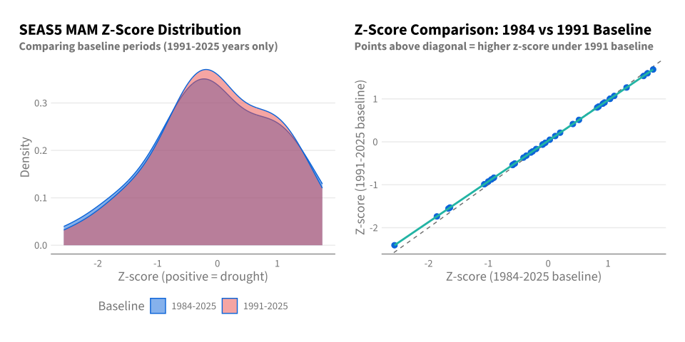
Trigger Performance Comparison
Three configurations: 1991 RP≥4, 1984 RP≥6, 1991 RP≥6
CDI Only (April) 1991, RP ≥ 4 1984, RP ≥ 6 1991, RP ≥ 6
CDI SEAS5 Combined SEAS5 Combined SEAS5 Combined
Evaluation period 42 (1984-2025) 35 (1991-2025) 35 (1991-2025) 42 (1984-2025) 42 (1984-2025) 35 (1991-2025) 35 (1991-2025)
Drought years 10 10 10 10 10 10 10
Years triggered 11 9 12 7 12 6 11
True positives 9 6 9 4 9 4 9
False positives 2 (2000, 2004) 3 (2000, 2004, 2010) 3 (2000, 2004, 2010) 3 (1985, 2000, 2004) 3 (1985, 2000, 2004) 2 (2000, 2004) 2 (2000, 2004)
Missed droughts 1 (2007) 4 (2007, 2011, 2022, 2025) 1 (2007) 6 (2007, 2011, 2021, 2022, 2023, 2025) 1 (2007) 6 (2007, 2011, 2021, 2022, 2023, 2025) 1 (2007)
Precision 0.82 0.67 0.75 0.57 0.75 0.67 0.82
Recall 0.9 0.6 0.9 0.4 0.9 0.4 0.9
F1 Score 0.86 0.63 0.82 0.47 0.82 0.5 0.86
Effective RP ~3.9 yr ~4 yr ~3 yr ~6.1 yr ~3.6 yr ~6 yr ~3.3 yr

C.8.4 SEAS5 Early Warning Value

Beyond standalone performance, SEAS5 adds value by providing one month earlier warning for droughts that CDI would eventually catch anyway.

Code
tibble(
    Metric = c(
        "Droughts with early warning",
        "Extra FP from SEAS5",
        "Early:FP ratio"
    ),
    Value = c(
        paste0(ew_1984_rp4_same$droughts_early, "/", ew_1984_rp4_same$total_droughts, " (", ew_1984_rp4_same$pct_early, "%)"),
        as.character(ew_1984_rp4_same$fp_added),
        paste0(ew_1984_rp4_same$ratio, ":1")
    )
) |>
    gt() |>
    tab_header(
        title = "SEAS5 Early Warning Value-Add",
        subtitle = "Additional benefit when used alongside CDI (1991-2025)"
    )
SEAS5 Early Warning Value-Add
Additional benefit when used alongside CDI (1991-2025)
Metric Value
Droughts with early warning 6/10 (60%)
Extra FP from SEAS5 1
Early:FP ratio 6:1
NoteInterpretation

CDI (April trigger) is the primary trigger with strong performance (evaluated on full 1984-2025 record):

  • Captures 90% of droughts (9/10)
  • Precision of 82% (2 false positive(s) in 42 years)
  • F1 score of 0.86

SEAS5 (March early warning) provides lead time options (evaluated on 1991-2025):

  • RP ≥ 4: Identifies 60% of droughts (6/10) with 1 FP(s) added beyond CDI
  • RP ≥ 6: Identifies 40% of droughts (4/10) with 0 FP(s) added beyond CDI

Combined trigger (CDI OR SEAS5) performance depends on SEAS5 threshold (evaluated on 1991-2025):

  • With SEAS5 RP ≥ 4: 90% recall, 75% precision, F1 = 0.82
  • With SEAS5 RP ≥ 6: 90% recall, 82% precision, F1 = 0.86