11  2026 Drought Trigger Modeling

11.1 Introduction

This chapter develops drought trigger models for anticipatory action in Afghanistan’s northern provinces. The core question: Can we predict end-of-season agricultural drought early enough to trigger humanitarian response?

We evaluate two potential trigger windows:

  • March publication: Earliest possible trigger, relies heavily on seasonal forecasts
  • April publication: One month later, incorporates early growing season observations

The fundamental trade-off: earlier triggers provide more lead time for response but have less observational data and thus lower accuracy.

ImportantKey Findings
  1. April window outperforms March due to growing-season observations
  2. March trigger: Use SEAS5 seasonal forecast alone - adding February observations hurts performance (F1=0.58 vs 0.47)
  3. April trigger: Use ridge-based CDI with interpretable component weights (LOOCV F1 ~0.82)
Code
box::use(
    dplyr[...],
    tidyr[...],
    ggplot2[...],
    gghdx[...],
    cumulus[...],
    purrr[...],
    glue[glue],
    tibble[tibble],
    ggfx[with_outer_glow],
    ggrepel[geom_text_repel],
    .. / R / utils[rp_empirical]
)

library(tidymodels)
gghdx()
Code
# Return period threshold for defining drought
RP_THRESHOLD <- 4

# Bootstrap resamples for cross-validation
N_BOOTSTRAP <- 30

# Random seed
SEED <- 42

# Feature set paths
FEATURE_PATHS <- list(
    march = "ds-aa-afg-drought/processed/vector/2026_mar_pub_feature_set_v1.parquet",
    april = "ds-aa-afg-drought/processed/vector/2026_april_pub_feature_set_v1.parquet"
)

# Variables to exclude per model variant
# Model 1 (Composite): uses mixed_fcast_obsv, excludes individual forecast components
APRIL_EXCLUDE_VARS <- c("total_precipitation_sum", "seas5 Apr", "seas5 May")
# Model 2 (Individual components): uses individual months, excludes composite
APRIL_EXCLUDE_VARS_MODEL2 <- c("mixed_fcast_obsv")
MARCH_EXCLUDE_VARS <- c()

11.2 Data Overview

11.2.1 Outcome Variable

We predict end-of-season agricultural drought, defined using the FAO Agricultural Stress Index (ASI) published in June (valid for May - end of growing season). Drought is defined empirically as years where ASI exceeds the 4-year return period threshold.

11.2.2 Predictors by Window

March publication (data valid for February):

  • ERA5-Land: snow cover, precipitation, soil moisture, cumulative precipitation
  • FAO: ASI, VHI (vegetation health)
  • SEAS5: Mar-Apr-May seasonal precipitation forecast

April publication (data valid for March):

  • Same ERA5-Land and FAO indicators (one month later)
  • SEAS5: April and May precipitation forecasts
  • mixed_fcast_obsv: Composite averaging observed March precip with forecasted Apr/May

All predictors are z-score standardized with sign convention: positive z-score = drought conditions.

Code
# Load feature sets
df_mar_raw <- blob_read(name = FEATURE_PATHS$march, container = "projects")
df_apr_raw <- blob_read(name = FEATURE_PATHS$april, container = "projects")

# Prepare modeling data with empirical RP thresholding
prepare_model_data <- function(df, rp_threshold = RP_THRESHOLD) {
    df |>
        filter(!is.na(outcome_asi_zscore)) |>
        arrange(desc(outcome_asi_zscore)) |>
        mutate(
            rank = row_number(),
            q_rank = rank / (n() + 1),
            rp_emp = 1 / q_rank,
            drought = factor(
                if_else(rp_emp >= rp_threshold, "yes", "no"),
                levels = c("yes", "no")
            )
        ) |>
        select(-outcome_asi_zscore, -rank, -q_rank, -rp_emp,
               -starts_with("adm0_name"), -pub_date, -timestep)
}

df_mar <- prepare_model_data(df_mar_raw)
df_apr <- prepare_model_data(df_apr_raw)

11.2.3 Sample Characteristics

Sample: 42 years (1984-2025) with 10 drought events (23.8%) at the 4-year return period threshold.

Code
bind_rows(
    df_mar |> count(drought) |> mutate(window = "March"),
    df_apr |> count(drought) |> mutate(window = "April")
) |>
    pivot_wider(names_from = drought, values_from = n) |>
    mutate(pct_drought = round(yes / (no + yes) * 100, 1)) |>
    knitr::kable(caption = "Class balance by trigger window")
Class balance by trigger window
window yes no pct_drought
March 10 32 23.8
April 10 32 23.8

11.3 Window Comparison: Why April Outperforms March

Before diving into model details, we establish a key finding: April indicators consistently outperform March indicators across all predictors.

Code
# Get predictor names
get_predictors <- function(data) {
    data |> select(-drought, -pub_year) |> colnames()
}

# Fit single-predictor logistic regression
fit_univariate <- function(data, predictor, n_boots = N_BOOTSTRAP, seed = SEED) {
    form <- as.formula(paste("drought ~", paste0("`", predictor, "`")))

    spec <- logistic_reg() |> set_engine("glm") |> set_mode("classification")
    wf <- workflow() |> add_recipe(recipe(form, data = data)) |> add_model(spec)

    set.seed(seed)
    boots <- bootstraps(data, times = n_boots, strata = drought)
    results <- fit_resamples(wf, resamples = boots,
                             control = control_resamples(save_pred = TRUE))
    preds <- collect_predictions(results)

    tibble(
        predictor = predictor,
        roc_auc = yardstick::roc_auc_vec(preds$drought, preds$.pred_yes),
        f_meas = yardstick::f_meas_vec(preds$drought, preds$.pred_class),
        precision = yardstick::precision_vec(preds$drought, preds$.pred_class),
        recall = yardstick::recall_vec(preds$drought, preds$.pred_class)
    )
}
Code
# Run for both windows
df_uni_apr <- map(get_predictors(df_apr), \(p) fit_univariate(df_apr, p)) |>
    list_rbind() |> mutate(window = "April")

df_uni_mar <- map(get_predictors(df_mar), \(p) fit_univariate(df_mar, p)) |>
    list_rbind() |> mutate(window = "March")

df_univariate <- bind_rows(df_uni_apr, df_uni_mar)
Code
df_univariate |>
    mutate(window = factor(window, levels = c("March", "April"))) |>
    ggplot(aes(x = window, y = reorder(predictor, f_meas), fill = f_meas)) +
    geom_tile(color = "white", linewidth = 0.5) +
    geom_text(aes(label = round(f_meas, 2)), color = "white", fontface = "bold") +
    scale_fill_gradient(low = "steelblue", high = "darkred", limits = c(0, 0.7)) +
    labs(
        title = "Univariate F1 Score by Predictor and Window",
        subtitle = "April consistently outperforms March across all indicators",
        x = NULL, y = NULL, fill = "F1"
    ) +
    theme(panel.grid = element_blank())

TipKey Finding: April Outperforms March

Every predictor shows higher univariate F1 score in the April window compared to March. This is expected: by April, we have observations from the early growing season (March) rather than pre-season data (February).

Note: These are screening metrics (bootstrap CV, default threshold) - see LOOCV section for honest multivariate performance estimates.

Code
df_univariate |>
    select(window, predictor, roc_auc, f_meas, precision, recall) |>
    arrange(window, desc(f_meas)) |>
    knitr::kable(
        digits = 3,
        caption = "Univariate predictor performance (bootstrap CV, default P > 0.5 threshold)",
        col.names = c("Window", "Predictor", "AUC", "F1", "Precision", "Recall")
    )
Univariate predictor performance (bootstrap CV, default P > 0.5 threshold)
Window Predictor AUC F1 Precision Recall
April mixed_fcast_obsv 0.874 0.601 0.721 0.516
April volumetric_soil_water_1m 0.853 0.594 0.650 0.547
April precip_cumsum 0.815 0.531 0.750 0.411
April asi 0.872 0.517 0.696 0.411
April seas5 May 0.813 0.500 0.558 0.453
April seas5 Apr 0.774 0.471 0.597 0.389
April total_precipitation_sum 0.770 0.435 0.530 0.368
April vhi 0.845 0.403 0.500 0.337
April snow_cover 0.741 0.382 0.484 0.316
March seas5 Mar-Apr-May 0.767 0.322 0.444 0.253
March asi 0.763 0.157 0.312 0.105
March vhi 0.723 0.132 0.308 0.084
March volumetric_soil_water_1m 0.667 0.119 0.304 0.074
March precip_cumsum 0.647 0.116 0.269 0.074
March snow_cover 0.661 0.110 0.429 0.063
March total_precipitation_sum 0.574 0.073 0.286 0.042

Note: Uses default P > 0.5 classification threshold. See Appendix C for tuned threshold analysis.

11.4 March Window: Forecast-Only Trigger

11.4.1 Physical Reasoning

For the March trigger window, predictor data is valid for February - before the growing season begins. Physically, we would expect:

  • SEAS5 forecast: Should be predictive (directly forecasts growing season precipitation)
  • February observations (ASI, VHI, soil moisture, snow): Less clear connection to end-of-season drought

We use Lasso regression to empirically test which variables are truly predictive. Lasso shrinks irrelevant coefficients to exactly zero, performing automatic feature selection.

11.4.2 Lasso Feature Selection

Code
# Lasso specification (mixture = 1 for pure L1 penalty)
lasso_spec <- logistic_reg(penalty = tune(), mixture = 1) |>
    set_engine("glmnet") |>
    set_mode("classification")

# Recipe for March data
lasso_recipe_mar <- recipe(drought ~ ., data = df_mar) |>
    step_rm(pub_year) |>
    step_zv(all_predictors())

lasso_wf_mar <- workflow() |>
    add_recipe(lasso_recipe_mar) |>
    add_model(lasso_spec)

# Tune penalty with bootstrap CV
set.seed(SEED)
lasso_boots <- bootstraps(df_mar, times = N_BOOTSTRAP, strata = drought)
lasso_grid <- grid_regular(penalty(range = c(-4, 0)), levels = 30)

lasso_tune_mar <- tune_grid(
    lasso_wf_mar,
    resamples = lasso_boots,
    grid = lasso_grid,
    metrics = metric_set(roc_auc, f_meas),
    control = control_grid(save_pred = TRUE)
)

# Select best penalty
best_lasso_penalty <- select_best(lasso_tune_mar, metric = "f_meas")

# Fit final model
final_lasso_mar <- lasso_wf_mar |>
    finalize_workflow(best_lasso_penalty) |>
    fit(data = df_mar)

# Extract coefficients
lasso_coefs_mar <- final_lasso_mar |>
    extract_fit_parsnip() |>
    tidy() |>
    filter(term != "(Intercept)") |>
    arrange(desc(abs(estimate)))
Code
lasso_coefs_mar |>
    mutate(
        selected = if_else(estimate != 0, "Yes", "No"),
        estimate = round(estimate, 4)
    ) |>
    select(term, estimate, selected) |>
    knitr::kable(
        caption = "March window: Lasso coefficients (non-zero = selected)",
        col.names = c("Predictor", "Coefficient", "Selected")
    )
March window: Lasso coefficients (non-zero = selected)
Predictor Coefficient Selected
seas5 Mar-Apr-May -1.3937 Yes
vhi -0.5805 Yes
snow_cover -0.5143 Yes
volumetric_soil_water_1m -0.3866 Yes
total_precipitation_sum 0.2251 Yes
precip_cumsum -0.0006 Yes
asi 0.0000 No

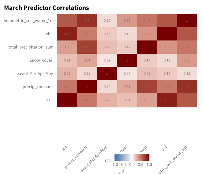
Result: SEAS5 Mar-Apr-May has the largest coefficient magnitude. Notably, ASI was dropped (coefficient = 0), suggesting February agricultural stress has no unique predictive value for June drought.

See Appendix A for the full correlation matrix and discussion of suppressor effects.

11.4.3 Model Comparison: SEAS5 vs Multivariate

We compare three approaches:

  1. SEAS5 only: Simple univariate model using just the seasonal forecast
  2. Lasso: Multivariate with automatic feature selection (all variables, L1 penalty)
  3. Ridge on lasso-selected: Two-stage approach - lasso for selection, ridge for stable coefficients
Code
# Univariate SEAS5 model
seas5_spec <- logistic_reg() |>
    set_engine("glm") |>
    set_mode("classification")

seas5_recipe <- recipe(drought ~ `seas5 Mar-Apr-May`, data = df_mar)

seas5_wf <- workflow() |>
    add_recipe(seas5_recipe) |>
    add_model(seas5_spec)

set.seed(SEED)
seas5_boots <- bootstraps(df_mar, times = N_BOOTSTRAP, strata = drought)

seas5_results <- fit_resamples(
    seas5_wf,
    resamples = seas5_boots,
    control = control_resamples(save_pred = TRUE)
)

seas5_preds <- collect_predictions(seas5_results)

# Tune threshold
seas5_thresh_results <- map_dfr(seq(0.1, 0.9, by = 0.05), function(thresh) {
    pred_class <- factor(
        if_else(seas5_preds$.pred_yes > thresh, "yes", "no"),
        levels = c("yes", "no")
    )
    tibble(
        threshold = thresh,
        f1 = f_meas_vec(seas5_preds$drought, pred_class),
        precision = precision_vec(seas5_preds$drought, pred_class),
        recall = recall_vec(seas5_preds$drought, pred_class)
    )
})

best_seas5_thresh <- seas5_thresh_results |>
    filter(f1 == max(f1, na.rm = TRUE)) |>
    slice(1)
Code
# Variables selected by lasso, excluding problematic ones
LASSO_SELECTED_VARS <- c("seas5 Mar-Apr-May", "vhi", "snow_cover",
                          "volumetric_soil_water_1m", "precip_cumsum")

# Ridge on lasso-selected variables
ridge_spec_mar <- logistic_reg(penalty = tune(), mixture = 0) |>
    set_engine("glmnet") |>
    set_mode("classification")

ridge_recipe_mar <- recipe(drought ~ ., data = df_mar) |>
    step_rm(pub_year) |>
    step_select(all_of(c("drought", LASSO_SELECTED_VARS))) |>
    step_zv(all_predictors())

ridge_wf_mar <- workflow() |>
    add_recipe(ridge_recipe_mar) |>
    add_model(ridge_spec_mar)

set.seed(SEED)
ridge_boots_mar <- bootstraps(df_mar, times = N_BOOTSTRAP, strata = drought)
penalty_grid_mar <- grid_regular(penalty(range = c(-4, 0)), levels = 30)

ridge_tune_mar <- tune_grid(
    ridge_wf_mar,
    resamples = ridge_boots_mar,
    grid = penalty_grid_mar,
    metrics = metric_set(roc_auc, f_meas, precision, recall),
    control = control_grid(save_pred = TRUE)
)

best_penalty_mar <- select_best(ridge_tune_mar, metric = "f_meas")

# Get metrics for comparison
ridge_mar_preds <- collect_predictions(ridge_tune_mar, parameters = best_penalty_mar)

ridge_mar_thresh_results <- map_dfr(seq(0.1, 0.9, by = 0.05), function(thresh) {
    pred_class <- factor(
        if_else(ridge_mar_preds$.pred_yes > thresh, "yes", "no"),
        levels = c("yes", "no")
    )
    tibble(
        threshold = thresh,
        f1 = f_meas_vec(ridge_mar_preds$drought, pred_class),
        precision = precision_vec(ridge_mar_preds$drought, pred_class),
        recall = recall_vec(ridge_mar_preds$drought, pred_class)
    )
})

best_ridge_mar_thresh <- ridge_mar_thresh_results |>
    filter(f1 == max(f1, na.rm = TRUE)) |>
    slice(1)

# Get lasso predictions for comparison
lasso_mar_preds <- collect_predictions(lasso_tune_mar, parameters = best_lasso_penalty)

lasso_mar_thresh_results <- map_dfr(seq(0.1, 0.9, by = 0.05), function(thresh) {
    pred_class <- factor(
        if_else(lasso_mar_preds$.pred_yes > thresh, "yes", "no"),
        levels = c("yes", "no")
    )
    tibble(
        threshold = thresh,
        f1 = f_meas_vec(lasso_mar_preds$drought, pred_class),
        precision = precision_vec(lasso_mar_preds$drought, pred_class),
        recall = recall_vec(lasso_mar_preds$drought, pred_class)
    )
})

best_lasso_mar_thresh <- lasso_mar_thresh_results |>
    filter(f1 == max(f1, na.rm = TRUE)) |>
    slice(1)
Code
tibble(
    Model = c("SEAS5 only", "Lasso (all variables)", "Ridge (lasso-selected)"),
    Threshold = c(best_seas5_thresh$threshold, best_lasso_mar_thresh$threshold, best_ridge_mar_thresh$threshold),
    F1 = c(best_seas5_thresh$f1, best_lasso_mar_thresh$f1, best_ridge_mar_thresh$f1),
    Precision = c(best_seas5_thresh$precision, best_lasso_mar_thresh$precision, best_ridge_mar_thresh$precision),
    Recall = c(best_seas5_thresh$recall, best_lasso_mar_thresh$recall, best_ridge_mar_thresh$recall)
) |>
    knitr::kable(
        digits = 3,
        caption = "March window model comparison (bootstrap CV, tuned thresholds)"
    )
March window model comparison (bootstrap CV, tuned thresholds)
Model Threshold F1 Precision Recall
SEAS5 only 0.3 0.577 0.479 0.726
Lasso (all variables) 0.4 0.436 0.397 0.484
Ridge (lasso-selected) 0.3 0.467 0.402 0.558
ImportantMarch Window Recommendation

Use SEAS5 seasonal forecast alone. The univariate SEAS5 model (F1=0.58) outperforms the multivariate model (F1=0.47).

Adding February observational data does not improve prediction - it adds noise rather than signal. This makes physical sense: pre-growing season observations have limited connection to end-of-season agricultural outcomes.

11.5 April Window: Combined Drought Index (CDI)

11.5.1 Available Data

By April publication, we have observations from March - the early growing season. This includes:

  • March precipitation: Critical for crop establishment
  • March soil moisture: Reflects accumulated water availability
  • March VHI/ASI: Early vegetation stress indicators
  • April/May forecasts: Remaining season precipitation outlook

The mixed_fcast_obsv composite (averaging observed March precip with forecasted Apr/May) performs best univariately.

11.5.2 Model Building: Ridge Regression

We use ridge regression rather than standard logistic regression because:

  1. Small sample size (n=42) with correlated predictors causes coefficient instability
  2. Ridge regularization shrinks coefficients toward zero, reducing variance
  3. Produces physically sensible weights (see Appendix B for GLM issues)
Code
fit_classification_model <- function(data, model_spec, exclude_vars = c("pub_year"),
                                      n_boots = N_BOOTSTRAP, seed = SEED) {
    recipe <- recipe(drought ~ ., data = data) |>
        step_rm(all_of(exclude_vars)) |>
        step_zv(all_predictors())

    workflow <- workflow() |> add_recipe(recipe) |> add_model(model_spec)

    set.seed(seed)
    boots <- bootstraps(data, times = n_boots, strata = drought)
    results <- fit_resamples(workflow, resamples = boots,
                             control = control_resamples(save_pred = TRUE))
    preds <- collect_predictions(results)

    metrics <- tibble(
        .metric = c("accuracy", "roc_auc", "f_meas", "precision", "recall"),
        mean = c(
            yardstick::accuracy_vec(preds$drought, preds$.pred_class),
            yardstick::roc_auc_vec(preds$drought, preds$.pred_yes),
            yardstick::f_meas_vec(preds$drought, preds$.pred_class),
            yardstick::precision_vec(preds$drought, preds$.pred_class),
            yardstick::recall_vec(preds$drought, preds$.pred_class)
        )
    )

    list(
        metrics = metrics,
        predictions = preds,
        final_fit = fit(workflow, data = data)
    )
}

get_logreg_coefs <- function(model_result) {
    model_result$final_fit |>
        extract_fit_parsnip() |>
        broom::tidy() |>
        filter(term != "(Intercept)") |>
        arrange(desc(abs(estimate)))
}
Code
# Ridge specification with penalty tuning
ridge_spec <- logistic_reg(penalty = tune(), mixture = 0) |>
    set_engine("glmnet") |>
    set_mode("classification")

# Recipe (data is already z-scored)
ridge_recipe <- recipe(drought ~ ., data = df_apr) |>
    step_rm(all_of(c("pub_year", APRIL_EXCLUDE_VARS, "precip_cumsum"))) |>
    step_zv(all_predictors())

ridge_wf <- workflow() |>
    add_recipe(ridge_recipe) |>
    add_model(ridge_spec)

# Bootstrap resampling with penalty tuning
set.seed(SEED)
ridge_boots <- bootstraps(df_apr, times = N_BOOTSTRAP, strata = drought)
penalty_grid <- grid_regular(penalty(range = c(-4, 0)), levels = 30)

ridge_tune <- tune_grid(
    ridge_wf,
    resamples = ridge_boots,
    grid = penalty_grid,
    metrics = metric_set(roc_auc, f_meas, precision, recall),
    control = control_grid(save_pred = TRUE)
)

# Select best penalty and finalize
best_penalty <- select_best(ridge_tune, metric = "f_meas")
final_ridge_wf <- ridge_wf |> finalize_workflow(best_penalty)
final_ridge_fit <- fit(final_ridge_wf, data = df_apr)

# Extract coefficients
coefs_ridge <- final_ridge_fit |>
    extract_fit_parsnip() |>
    tidy() |>
    filter(term != "(Intercept)")

# CDI weights: negate because parsnip/glmnet convention
cdi_weights <- coefs_ridge |>
    mutate(
        weight = -estimate / sum(abs(estimate)),
        contribution_pct = abs(weight) * 100
    ) |>
    arrange(desc(contribution_pct)) |>
    select(term, estimate, weight, contribution_pct)

11.5.3 CDI Construction

The Combined Drought Index (CDI) is a weighted sum of standardized indicators, with weights derived from ridge regression coefficients:

Code
cdi_weights |>
    knitr::kable(
        digits = 3,
        col.names = c("Indicator", "Ridge Coef", "CDI Weight", "Contribution %"),
        caption = "CDI weights derived from ridge regression"
    )
CDI weights derived from ridge regression
Indicator Ridge Coef CDI Weight Contribution %
mixed_fcast_obsv -0.741 0.275 27.545
asi -0.554 0.206 20.608
snow_cover -0.552 0.205 20.537
vhi -0.516 0.192 19.190
volumetric_soil_water_1m -0.326 0.121 12.120
Code
formula_parts <- cdi_weights |>
    arrange(desc(weight)) |>
    mutate(
        part = paste0(
            if_else(row_number() == 1, "", " + "),
            round(weight, 3), " × ", term
        )
    ) |>
    pull(part)

cat("**CDI Formula:**\n\n$$\\text{CDI} = ", paste(formula_parts, collapse = ""), "$$\n")

CDI Formula:

\[\text{CDI} = 0.275 × mixed_fcast_obsv + 0.206 × asi + 0.205 × snow_cover + 0.192 × vhi + 0.121 × volumetric_soil_water_1m \]

Interpretation: Higher CDI values indicate higher drought risk. The weights reflect each indicator’s predictive contribution - VHI and the mixed forecast/observation composite contribute most.

Code
calc_cdi <- function(data, weights_df) {
    cdi <- rep(0, nrow(data))
    for (i in seq_len(nrow(weights_df))) {
        feat <- weights_df$term[i]
        w <- weights_df$weight[i]
        if (feat %in% colnames(data)) {
            cdi <- cdi + w * data[[feat]]
        }
    }
    cdi
}

df_apr_cdi <- df_apr |>
    mutate(
        CDI = calc_cdi(df_apr, cdi_weights),
        year = pub_year
    )

# CDI empirical RPs (Weibull plotting position) — trigger threshold
# is derived from F1-optimized probability in the threshold-analysis chunk
df_apr_cdi <- df_apr_cdi |>
    mutate(cdi_rp = rp_empirical(CDI, direction = "-1"))

11.6 Threshold Selection

11.6.1 The Problem

Our model outputs continuous values (CDI or predicted probabilities). We need a threshold to convert these to yes/no trigger decisions. Three approaches:

  1. Default P > 0.5: Standard classification threshold
  2. F1-optimized threshold: Probability threshold that maximizes F1 score
  3. CDI (F1-equivalent): The CDI value equivalent to the F1-optimized probability threshold, expressed as a Weibull percentile/RP
Code
# Get predicted probabilities
df_apr_probs <- df_apr_cdi |>
    mutate(
        prob_drought = predict(final_ridge_fit, df_apr, type = "prob")$.pred_yes,
        trigger_default = factor(
            if_else(prob_drought > 0.5, "yes", "no"),
            levels = c("yes", "no")
        )
    )

# Tune threshold for F1
thresholds <- seq(0.1, 0.9, by = 0.05)

threshold_results <- map_dfr(thresholds, function(thresh) {
    pred <- factor(
        if_else(df_apr_probs$prob_drought > thresh, "yes", "no"),
        levels = c("yes", "no")
    )

    tibble(
        threshold = thresh,
        precision = precision_vec(df_apr_probs$drought, pred),
        recall = recall_vec(df_apr_probs$drought, pred),
        f1 = f_meas_vec(df_apr_probs$drought, pred),
        n_triggered = sum(pred == "yes")
    )
})

best_prob_threshold <- threshold_results |>
    filter(f1 == max(f1, na.rm = TRUE)) |>
    slice(1) |>
    pull(threshold)

# Derive CDI threshold from F1-optimized probability
# Since CDI and probability rankings are identical (same model, monotonic transform),
# the F1-optimized probability maps to a specific CDI cutoff
n_trigger_tuned <- sum(df_apr_probs$prob_drought > best_prob_threshold)
cdi_threshold <- min(df_apr_probs$CDI[df_apr_probs$prob_drought > best_prob_threshold])

# Weibull RP and percentile equivalent of the F1-optimized threshold
rp_f1_equivalent <- round((nrow(df_apr_probs) + 1) / n_trigger_tuned, 2)
weibull_pctile <- round((1 - n_trigger_tuned / (nrow(df_apr_probs) + 1)) * 100, 1)

df_apr_compare <- df_apr_probs |>
    mutate(
        trigger_tuned = factor(
            if_else(prob_drought > best_prob_threshold, "yes", "no"),
            levels = c("yes", "no")
        ),
        trigger = factor(
            if_else(CDI >= cdi_threshold, "yes", "no"),
            levels = c("yes", "no")
        )
    )

# Update df_apr_cdi for downstream use (plots, confusion matrix)
df_apr_cdi <- df_apr_cdi |>
    mutate(
        trigger = factor(if_else(CDI >= cdi_threshold, "yes", "no"),
                         levels = c("yes", "no"))
    )
Code
threshold_results |>
    pivot_longer(cols = c(precision, recall, f1),
                 names_to = "metric", values_to = "value") |>
    ggplot(aes(x = threshold, y = value, color = metric)) +
    geom_line(linewidth = 1) +
    geom_point(size = 2) +
    geom_vline(xintercept = best_prob_threshold, linetype = "dashed") +
    geom_vline(xintercept = 0.5, linetype = "dotted", color = "gray") +
    annotate("text", x = best_prob_threshold + 0.03, y = 0.3,
             label = paste0("F1-optimal: ", best_prob_threshold), hjust = 0) +
    scale_color_manual(values = c("precision" = "steelblue", "recall" = "tomato", "f1" = "darkgreen")) +
    labs(
        title = "Probability Threshold Tuning",
        subtitle = "Dashed = F1-optimal | Dotted = default 0.5",
        x = "Probability Threshold", y = "Metric Value", color = "Metric"
    )

11.6.2 Three-Way Comparison

Code
calc_trigger_metrics <- function(pred, actual) {
    pred_f <- factor(pred, levels = c("yes", "no"))
    tibble(
        precision = precision_vec(actual, pred_f),
        recall = recall_vec(actual, pred_f),
        f1 = f_meas_vec(actual, pred_f),
        n_triggered = sum(pred_f == "yes")
    )
}

comparison_table <- bind_rows(
    calc_trigger_metrics(df_apr_compare$trigger_default, df_apr_compare$drought) |>
        mutate(approach = "P > 0.5 (default)", threshold = "0.50"),
    calc_trigger_metrics(df_apr_compare$trigger_tuned, df_apr_compare$drought) |>
        mutate(approach = "P > tuned (F1)", threshold = as.character(best_prob_threshold)),
    calc_trigger_metrics(df_apr_compare$trigger, df_apr_compare$drought) |>
        mutate(
            approach = "CDI (F1-equivalent)",
            threshold = glue("CDI ≥ {round(cdi_threshold, 3)} ({weibull_pctile}th %ile)")
        )
) |>
    select(approach, threshold, precision, recall, f1, n_triggered)

comparison_table |>
    knitr::kable(
        digits = 3,
        col.names = c("Approach", "Threshold", "Precision", "Recall", "F1", "N Triggered"),
        caption = "Comparison of trigger approaches - April window (in-sample)"
    )
Comparison of trigger approaches - April window (in-sample)
Approach Threshold Precision Recall F1 N Triggered
P > 0.5 (default) 0.50 0.857 0.6 0.706 7
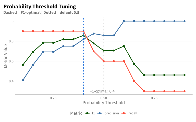
P > tuned (F1) 0.4 0.818 0.9 0.857 11
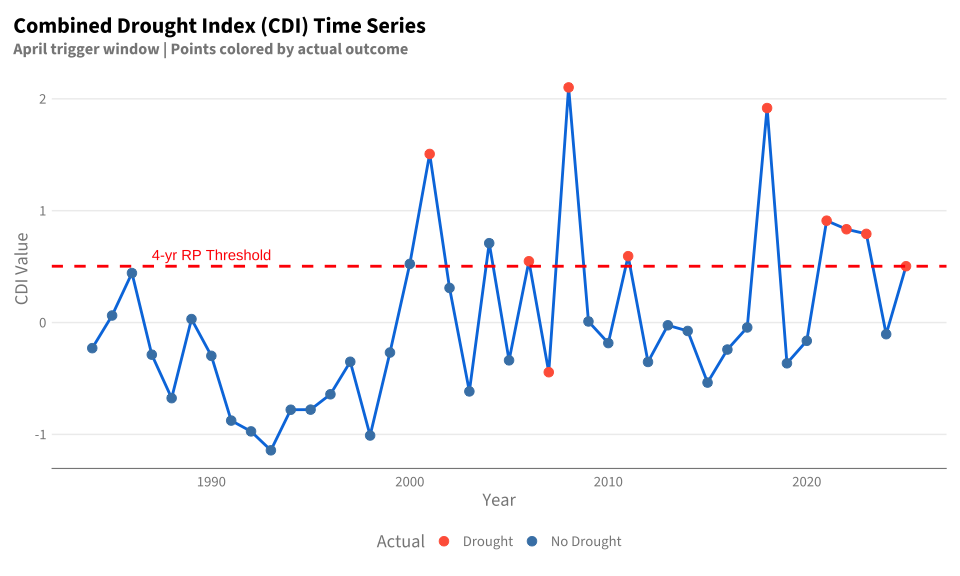
CDI (F1-equivalent) CDI ≥ 0.503 (74.4th %ile) 0.818 0.9 0.857 11

Ranking equivalence: Since CDI is derived from the same model, probability and CDI rankings are identical (correlation = 1). The F1-optimized probability threshold (P > 0.4) maps exactly to CDI ≥ 0.503 — both trigger 11 years.

NoteThreshold Equivalence

The F1-optimized threshold (P > 0.4) triggers 11 of 42 years (26.2%), corresponding to the 74.4th percentile (Weibull plotting position: rank/(n+1)), or equivalently a return period of 3.91 years.

This is close to the policy target of RP4 (75th percentile). The statistically optimal threshold approximately recovers the operationally desired trigger frequency.

11.7 Model Validation (LOOCV)

In-sample metrics are overly optimistic. For honest performance estimates, we use Leave-One-Out Cross-Validation (LOOCV): for each year, we fit the model on all other years and predict the held-out year.

Critically, we re-derive CDI weights and thresholds for each fold - this ensures truly out-of-sample evaluation.

Code
# LOOCV for ridge-based CDI
loocv_ridge_results <- map_dfr(1:nrow(df_apr), function(i) {
    train <- df_apr[-i, ]
    test <- df_apr[i, ]

    ridge_recipe_loo <- recipe(drought ~ ., data = train) |>
        step_rm(all_of(c("pub_year", APRIL_EXCLUDE_VARS, "precip_cumsum"))) |>
        step_zv(all_predictors())

    ridge_spec_loo <- logistic_reg(penalty = best_penalty$penalty, mixture = 0) |>
        set_engine("glmnet") |>
        set_mode("classification")

    ridge_wf_loo <- workflow() |>
        add_recipe(ridge_recipe_loo) |>
        add_model(ridge_spec_loo)

    fit_result <- fit(ridge_wf_loo, data = train)

    coefs <- fit_result |>
        extract_fit_parsnip() |>
        tidy() |>
        filter(term != "(Intercept)")

    weights <- coefs |>
        mutate(weight = -estimate / sum(abs(estimate)))

    # Calculate CDI for training data to get threshold
    train_cdi <- rep(0, nrow(train))
    for (j in seq_len(nrow(weights))) {
        feat <- weights$term[j]
        w <- weights$weight[j]
        if (feat %in% colnames(train)) {
            train_cdi <- train_cdi + w * train[[feat]]
        }
    }
    train_rp <- rp_empirical(train_cdi, direction = "-1")
    threshold <- min(train_cdi[train_rp >= RP_THRESHOLD])

    # Calculate CDI for test observation
    test_cdi <- 0
    for (j in seq_len(nrow(weights))) {
        feat <- weights$term[j]
        w <- weights$weight[j]
        if (feat %in% colnames(test)) {
            test_cdi <- test_cdi + w * test[[feat]]
        }
    }

    tibble(
        year = test$pub_year,
        actual = as.character(test$drought),
        cdi = test_cdi,
        threshold = threshold,
        predicted = if_else(test_cdi >= threshold, "yes", "no")
    )
})

# Calculate Ridge LOOCV metrics
loocv_ridge_conf <- table(
    Predicted = factor(loocv_ridge_results$predicted, levels = c("yes", "no")),
    Actual = factor(loocv_ridge_results$actual, levels = c("yes", "no"))
)

tp_ridge_loo <- loocv_ridge_conf["yes", "yes"]
fp_ridge_loo <- loocv_ridge_conf["yes", "no"]
fn_ridge_loo <- loocv_ridge_conf["no", "yes"]
tn_ridge_loo <- loocv_ridge_conf["no", "no"]
Code
# In-sample metrics for comparison
conf_mat <- table(Trigger = df_apr_cdi$trigger, Actual = df_apr_cdi$drought)
tp <- conf_mat["yes", "yes"]
fp <- conf_mat["yes", "no"]
fn <- conf_mat["no", "yes"]
tn <- conf_mat["no", "no"]

tibble(
    Metric = c("Precision", "Recall", "F1 Score", "Years Triggered"),
    `In-Sample` = c(
        round(tp / (tp + fp), 3),
        round(tp / (tp + fn), 3),
        round(2 * tp / (2 * tp + fp + fn), 3),
        tp + fp
    ),
    `LOOCV` = c(
        round(tp_ridge_loo / (tp_ridge_loo + fp_ridge_loo), 3),
        round(tp_ridge_loo / (tp_ridge_loo + fn_ridge_loo), 3),
        round(2 * tp_ridge_loo / (2 * tp_ridge_loo + fp_ridge_loo + fn_ridge_loo), 3),
        tp_ridge_loo + fp_ridge_loo
    )
) |>
    knitr::kable(caption = "In-sample vs LOOCV performance (Ridge)")
In-sample vs LOOCV performance (Ridge)
Metric In-Sample LOOCV
Precision 0.818 0.727
Recall 0.900 0.800
F1 Score 0.857 0.762
Years Triggered 11.000 11.000
Code
loocv_ridge_conf |>
    as.data.frame.matrix() |>
    knitr::kable(caption = "LOOCV confusion matrix (Ridge)")
LOOCV confusion matrix (Ridge)
yes no
yes 8 3
no 2 29

LOOCV results are the honest performance estimates - these are the numbers to report for expected trigger performance.

11.8 Visualization & Interpretation

11.8.1 CDI Time Series

Code
ggplot(df_apr_cdi, aes(x = year, y = CDI)) +
    geom_line(linewidth = 1) +
    geom_point(aes(color = drought), size = 3) +
    geom_hline(yintercept = cdi_threshold, linetype = "dashed",
               color = "red", linewidth = 1) +
    scale_color_manual(
        values = c("yes" = "tomato", "no" = "steelblue"),
        labels = c("yes" = "Drought", "no" = "No Drought")
    ) +
    annotate("text", x = min(df_apr_cdi$year) + 3, y = cdi_threshold + 0.1,
             label = paste0(RP_THRESHOLD, "-yr RP Threshold"),
             hjust = 0, color = "red") +
    labs(
        title = "Combined Drought Index (CDI) Time Series",
        subtitle = "April trigger window | Points colored by actual outcome",
        x = "Year", y = "CDI Value", color = "Actual"
    )

11.8.2 Component Contributions

Code
# Color palette matching monitoring plot style
pal_components <- c(
    "CDI" = "black",
    "VHI" = "#CCEBC5",
    "MAM precip (mixed obs forecast)" = "#DECBE4",
    "Snow Cover" = "#FFFF90",
    "ASI" = "#FBB4AE",
    "Soil moisture" = "#fec44f"
)

# Map component names to nice labels
component_label_map <- c(
    "vhi" = "VHI",
    "mixed_fcast_obsv" = "MAM precip (mixed obs forecast)",
    "snow_cover" = "Snow Cover",
    "asi" = "ASI",
    "volumetric_soil_water_1m" = "Soil moisture"
)

df_components <- df_apr_cdi |>
    select(year, drought, all_of(cdi_weights$term), CDI) |>
    pivot_longer(cols = all_of(cdi_weights$term),
                 names_to = "component", values_to = "zscore") |>
    mutate(
        parameter_label = component_label_map[component],
        parameter_label = factor(parameter_label, levels = names(pal_components))
    )

# CDI data for separate layer
df_cdi_line <- df_apr_cdi |>
    mutate(parameter_label = "CDI")

# Drought years for points and labels
df_drought_years <- df_apr_cdi |>
    filter(drought == "yes")

p_cdi_components <- ggplot() +
    # Component lines with shadow
    ggfx::with_shadow(
        geom_line(
            data = df_components,
            aes(x = year, y = zscore, color = parameter_label, group = parameter_label),
            alpha = 1, linewidth = 0.5
        ),
        sigma = 1.0, x_offset = 0.5, y_offset = 0.25
    ) +
    # Threshold line
    geom_hline(
        yintercept = cdi_threshold,
        color = hdx_hex("tomato-dark"),
        linetype = "dashed", linewidth = 0.5
    ) +
    # CDI line with shadow (on top)
    ggfx::with_shadow(
        geom_line(
            data = df_cdi_line,
            aes(x = year, y = CDI),
            color = "black", linewidth = 1
        ),
        sigma = 2, x_offset = 0.5, y_offset = 0.25
    ) +
    # Drought year points
    geom_point(
        data = df_drought_years,
        aes(x = year, y = CDI),
        color = hdx_hex("tomato-hdx"),
        size = 2.5, alpha = 0.7
    ) +
    # Threshold label
    geom_label(
        aes(x = 1990, y = cdi_threshold,
            label = paste0("Threshold: ", round(cdi_threshold, 2))),
        vjust = -0.3, hjust = 0,
        color = hdx_hex("tomato-dark"),
        size = 4, alpha = 0.5,
        label.padding = unit(0.15, "cm")
    ) +
    # Year labels for drought years
    geom_text_repel(
        data = df_drought_years,
        aes(x = year, y = CDI, label = year),
        color = hdx_hex("tomato-hdx"),
        vjust = -2, size = 3.5, alpha = 1
    ) +
    # Scales
    scale_color_manual(values = pal_components, drop = FALSE, name = NULL) +
    scale_x_continuous(
        breaks = seq(1985, 2025, by = 5),
        expand = expansion(mult = c(0.01, 0.03))
    ) +
    # Labels
    labs(
        title = "Drought AA Afghanistan: 2026 April Trigger",
        subtitle = "Red dashed line represents RP 4 threshold",
        x = NULL,
        y = "Indicator anomaly"
    ) +
    theme(
        axis.title.x = element_blank(),
        axis.title.y = element_text(size = 14),
        title = element_text(size = 16),
        legend.key.width = unit(1, "cm"),
        plot.subtitle = element_text(size = 14, color = "grey40"),
        legend.title = element_blank(),
        legend.text = element_text(size = 12),
        legend.position = "bottom",
        axis.text.y = element_text(angle = 90, size = 10, hjust = 0.5),
        axis.text.x = element_text(size = 10),
        panel.grid.minor = element_blank(),
        panel.grid.major.x = element_blank()
    ) +
    guides(color = guide_legend(nrow = 1, override.aes = list(linewidth = 2)))

ggsave("outputs/figures/fig-cdi-components.png", p_cdi_components, width = 10, height = 6, dpi = 300)

# Paper version with larger text
p_cdi_components_paper <- p_cdi_components +
    theme(
        axis.title.y = element_text(size = 16),
        title = element_text(size = 18),
        plot.subtitle = element_text(size = 16, color = "grey40"),
        legend.text = element_text(size = 14),
        axis.text.y = element_text(angle = 90, size = 12, hjust = 0.5),
        axis.text.x = element_text(size = 12)
    )
ggsave("outputs/figures/paper/fig-cdi-components.png", p_cdi_components_paper, width = 10, height = 6, dpi = 300)

p_cdi_components
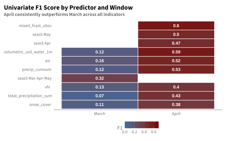
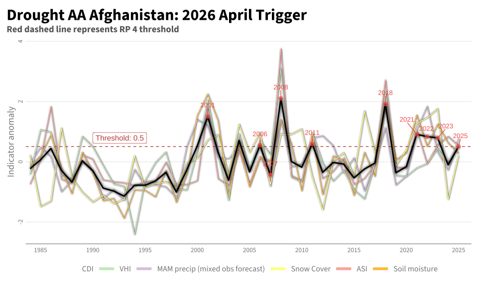
Figure 11.1: CDI Components and Weighted Index

11.8.3 Year-by-Year Trigger Decisions

Code
library(gt)

df_apr_compare |>
    select(year, drought, prob_drought, CDI, trigger_default, trigger_tuned, trigger) |>
    arrange(desc(prob_drought)) |>
    rename(
        Year = year,
        Actual = drought,
        `P(drought)` = prob_drought,
        `P>0.5` = trigger_default,
        `P>tuned` = trigger_tuned,
        `CDI tuned` = trigger
    ) |>
    gt() |>
    tab_header(
        title = "Trigger Comparison: April Window (All Years)",
        subtitle = "Sorted by predicted drought probability"
    ) |>
    fmt_number(columns = c(`P(drought)`, CDI), decimals = 3) |>
    tab_style(
        style = cell_fill(color = "tomato", alpha = 0.4),
        locations = cells_body(columns = Actual, rows = Actual == "yes")
    ) |>
    tab_style(
        style = cell_fill(color = "steelblue", alpha = 0.4),
        locations = cells_body(columns = `P>0.5`, rows = `P>0.5` == "yes")
    ) |>
    tab_style(
        style = cell_fill(color = "steelblue", alpha = 0.4),
        locations = cells_body(columns = `P>tuned`, rows = `P>tuned` == "yes")
    ) |>
    tab_style(
        style = cell_fill(color = "steelblue", alpha = 0.4),
        locations = cells_body(columns = `CDI tuned`, rows = `CDI tuned` == "yes")
    ) |>
    tab_spanner(
        label = "Trigger Decision",
        columns = c(`P>0.5`, `P>tuned`, `CDI tuned`)
    ) |>
    tab_footnote(
        footnote = "Red = actual drought | Blue = triggered",
        locations = cells_column_spanners()
    )
Table 11.1: Trigger Comparison: April Window (All Years)
Trigger Comparison: April Window (All Years)
Sorted by predicted drought probability
Year Actual P(drought) CDI Trigger Decision1
P>0.5 P>tuned CDI tuned
2008 yes 0.981 2.102 yes yes yes
2018 yes 0.970 1.917 yes yes yes
2001 yes 0.914 1.507 yes yes yes
2021 yes 0.680 0.911 yes yes yes
2022 yes 0.634 0.834 yes yes yes
2023 yes 0.608 0.793 yes yes yes
2004 no 0.553 0.709 yes yes yes
2011 yes 0.476 0.593 no yes yes
2006 yes 0.445 0.548 no yes yes
2000 no 0.430 0.524 no yes yes
2025 yes 0.416 0.503 no yes yes
1986 no 0.377 0.442 no no no
2002 no 0.297 0.309 no no no
1985 no 0.179 0.063 no no no
1989 no 0.167 0.031 no no no
2009 no 0.159 0.010 no no no
2013 no 0.147 −0.025 no no no
2017 no 0.141 −0.044 no no no
2014 no 0.131 −0.075 no no no
2024 no 0.122 −0.104 no no no
2020 no 0.106 −0.163 no no no
2010 no 0.101 −0.184 no no no
1984 no 0.090 −0.229 no no no
2016 no 0.088 −0.241 no no no
1999 no 0.082 −0.268 no no no
1987 no 0.078 −0.287 no no no
1990 no 0.076 −0.298 no no no
2005 no 0.069 −0.338 no no no
1997 no 0.067 −0.351 no no no
2012 no 0.067 −0.352 no no no
2019 no 0.065 −0.364 no no no
2007 yes 0.053 −0.444 no no no
2015 no 0.042 −0.537 no no no
2003 no 0.034 −0.616 no no no
1996 no 0.032 −0.641 no no no
1988 no 0.029 −0.676 no no no
1995 no 0.022 −0.779 no no no
1994 no 0.022 −0.779 no no no
1991 no 0.017 −0.876 no no no
1992 no 0.013 −0.973 no no no
1998 no 0.012 −1.010 no no no
1993 no 0.008 −1.142 no no no
1 Red = actual drought | Blue = triggered

11.9 Summary & Recommendations

ImportantRecommendations for 2026 Trigger

March Window (if earlier trigger needed):

  • Use SEAS5 seasonal forecast only
  • Simpler and performs better than multivariate (F1=0.58 vs 0.47)
  • February observations add noise, not signal

April Window (recommended):

  • Use ridge-based CDI with 4-year return period threshold
  • Interpretable component weights: VHI (19%), mixed_fcast_obsv (28%), snow_cover (21%), asi (21%)

Expected Performance (LOOCV estimates):

  • Precision: 73%
  • Recall: 80%
  • F1: 0.76
Code
cat("**CDI Weights:**\n\n")

CDI Weights:

Code
cdi_weights |>
    mutate(text = paste0("- **", term, "**: ", round(weight * 100, 1), "%")) |>
    pull(text) |>
    cat(sep = "\n")
  • mixed_fcast_obsv: 27.5%
  • asi: 20.6%
  • snow_cover: 20.5%
  • vhi: 19.2%
  • volumetric_soil_water_1m: 12.1%

11.10 Methodological Note: Ridge Regression vs Grid Search

This year’s approach differs from the 2025 analysis. This section documents the methodological choices and their trade-offs.

11.10.2 This Year’s Approach: Regularized Regression with LOOCV

The 2026 analysis uses ridge regression:

  1. Model fitting: Ridge regression (L2 penalty) learns weights from predictor-outcome relationships
  2. Regularization: Penalty term shrinks coefficients toward zero, trading bias for variance reduction
  3. Tuning: Penalty strength selected via bootstrap cross-validation
  4. Validation: Final performance estimated via leave-one-out cross-validation (LOOCV)

Strengths:

  • Honest out-of-sample estimates: LOOCV provides unbiased performance estimates
  • Regularization controls overfitting: Penalty term prevents fitting to noise
  • Principled variable weighting: Weights emerge from data relationships, not exhaustive search
  • Feature selection via lasso: L1 penalty identifies truly predictive variables before ridge fitting

Limitations:

  • Weights emerge from model fitting rather than explicit analyst choices (though easily normalized to proportions)
  • Requires familiarity with regularization concepts

11.10.3 Comparison Caveats

Direct F1 comparison between the two approaches is not straightforward:

  • 2025: Modeled at province level (separate CDI per province), with some provinces achieving F1 ~0.8
  • 2026: Models the merged 5-province area as a single unit (area-weighted mean of indicators)

These are different prediction problems. The merged approach trades spatial granularity for a more stable signal and simpler operational trigger (one threshold for the entire region rather than five).

11.10.4 Key Differences in Interpretation

The critical difference is confidence in the estimates:

Aspect Grid Search (2025) Ridge + LOOCV (2026)
Performance estimate Likely optimistic (in-sample) Honest (out-of-sample)
Degrees of freedom ~200,000 combinations tested ~10 hyperparameters
Overfitting risk High Low (regularized)
Generalization Uncertain More reliable

11.10.5 Weight Comparison

Code
# 2025 weights (from design_weights() / weight set 11209)
df_weights_2025 <- tibble(
    indicator = c("Snow Cover", "Precip Cumsum", "Soil Moisture",
                  "MAM Precip (mixed)", "ASI", "VHI"),
    weight = c(0.15, 0.05, 0.05, 0.25, 0.25, 0.25),
    model = "2025"
)

# 2026 weights from ridge regression (live from cdi_weights)
indicator_label_map <- c(
    "vhi" = "VHI",
    "mixed_fcast_obsv" = "MAM Precip (mixed)",
    "snow_cover" = "Snow Cover",
    "asi" = "ASI",
    "volumetric_soil_water_1m" = "Soil Moisture"
)

df_weights_2026 <- cdi_weights |>
    mutate(
        indicator = indicator_label_map[term],
        model = "2026"
    ) |>
    select(indicator, weight, model)

# Combine
df_weights_all <- bind_rows(df_weights_2025, df_weights_2026) |>
    mutate(
        indicator = factor(indicator, levels = c(
            "VHI", "ASI", "MAM Precip (mixed)",
            "Snow Cover", "Soil Moisture", "Precip Cumsum"
        )),
        pct_label = paste0(round(weight * 100, 0), "%")
    )

pal_indicators <- c(
    "VHI" = "#CCEBC5",
    "ASI" = "#FBB4AE",
    "MAM Precip (mixed)" = "#DECBE4",
    "Snow Cover" = "#FFFF90",
    "Soil Moisture" = "#fec44f",
    "Precip Cumsum" = "#B3CDE3"
)

ggplot(df_weights_all, aes(x = model, y = weight, fill = indicator)) +
    geom_col(width = 0.6, color = "grey30", linewidth = 0.3) +
    geom_text(
        aes(label = pct_label),
        position = position_stack(vjust = 0.5),
        size = 3.5, fontface = "bold"
    ) +
    scale_fill_manual(values = pal_indicators, drop = FALSE) +
    scale_y_continuous(labels = scales::percent, expand = c(0, 0)) +
    labs(
        title = "CDI Component Weights: 2025 vs 2026",
        subtitle = "2025: grid search | 2026: ridge regression",
        x = NULL, y = "Weight", fill = "Indicator"
    ) +
    theme(
        legend.position = "right",
        panel.grid.major.x = element_blank()
    )

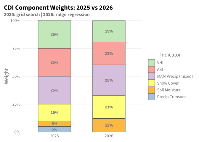
The 2026 model drops precip_cumsum (redundant with other precipitation indicators — see Appendix F) and redistributes weight toward soil moisture and snow cover. The precipitation composite and VHI/ASI remain the dominant contributors in both years.

NoteBottom Line

The 2025 grid search likely found real signal, but performance estimates are optimistically biased due to in-sample optimization. The 2026 ridge approach provides more defensible estimates of true out-of-sample performance through LOOCV validation and regularization. The methodological differences (province-level vs merged area) mean direct F1 comparison is not meaningful.


11.11 Appendix E: Composite vs Individual Forecast Components

The main CDI model uses mixed_fcast_obsv — an equal-weighted average of observed March precipitation, forecasted April, and forecasted May. A natural question: does letting the model weight these three months individually improve performance?

We fit a second ridge model that replaces mixed_fcast_obsv with total_precipitation_sum, seas5 Apr, and seas5 May as separate features, then compare LOOCV performance.

Code
# Model 2: individual forecast components
ridge_recipe_m2 <- recipe(drought ~ ., data = df_apr) |>
    step_rm(all_of(c("pub_year", APRIL_EXCLUDE_VARS_MODEL2, "precip_cumsum"))) |>
    step_zv(all_predictors())

ridge_wf_m2 <- workflow() |>
    add_recipe(ridge_recipe_m2) |>
    add_model(ridge_spec)

set.seed(SEED)
ridge_boots_m2 <- bootstraps(df_apr, times = N_BOOTSTRAP, strata = drought)

ridge_tune_m2 <- tune_grid(
    ridge_wf_m2,
    resamples = ridge_boots_m2,
    grid = penalty_grid,
    metrics = metric_set(roc_auc, f_meas, precision, recall),
    control = control_grid(save_pred = TRUE)
)

best_penalty_m2 <- select_best(ridge_tune_m2, metric = "f_meas")
final_ridge_fit_m2 <- fit(
    ridge_wf_m2 |> finalize_workflow(best_penalty_m2),
    data = df_apr
)

coefs_ridge_m2 <- final_ridge_fit_m2 |>
    extract_fit_parsnip() |>
    tidy() |>
    filter(term != "(Intercept)")

cdi_weights_m2 <- coefs_ridge_m2 |>
    mutate(
        weight = -estimate / sum(abs(estimate)),
        contribution_pct = abs(weight) * 100
    ) |>
    arrange(desc(contribution_pct)) |>
    select(term, estimate, weight, contribution_pct)

11.11.1 Learned Weights

Ridge does not weight the three months equally:

Code
cdi_weights_m2 |>
    knitr::kable(
        digits = 3,
        col.names = c("Indicator", "Ridge Coef", "CDI Weight", "Contribution %"),
        caption = "CDI weights — individual components model"
    )
CDI weights — individual components model
Indicator Ridge Coef CDI Weight Contribution %
snow_cover -0.571 0.202 20.199
asi -0.539 0.191 19.056
vhi -0.521 0.184 18.420
seas5 Apr -0.503 0.178 17.767
volumetric_soil_water_1m -0.324 0.115 11.453
seas5 May -0.216 0.076 7.633
total_precipitation_sum -0.155 0.055 5.472

The April forecast receives ~3x the weight of observed March precipitation or May forecast. However, the total precipitation-related contribution (~31%) is similar to the composite’s weight (~28%) — the other indicators absorb the difference.

11.11.2 LOOCV Comparison

Code
# LOOCV for model 2
loocv_m2_results <- map_dfr(1:nrow(df_apr), function(i) {
    train <- df_apr[-i, ]
    test <- df_apr[i, ]

    rec <- recipe(drought ~ ., data = train) |>
        step_rm(all_of(c("pub_year", APRIL_EXCLUDE_VARS_MODEL2, "precip_cumsum"))) |>
        step_zv(all_predictors())
    spec <- logistic_reg(penalty = best_penalty_m2$penalty, mixture = 0) |>
        set_engine("glmnet") |> set_mode("classification")
    wf <- workflow() |> add_recipe(rec) |> add_model(spec)
    fit_result <- fit(wf, data = train)

    # Get probability for ROC AUC
    prob <- predict(fit_result, test, type = "prob")$.pred_yes

    # CDI-based trigger
    coefs <- fit_result |> extract_fit_parsnip() |> tidy() |>
        filter(term != "(Intercept)") |>
        mutate(weight = -estimate / sum(abs(estimate)))

    train_cdi <- rep(0, nrow(train))
    for (j in seq_len(nrow(coefs))) {
        feat <- coefs$term[j]; w <- coefs$weight[j]
        if (feat %in% colnames(train)) train_cdi <- train_cdi + w * train[[feat]]
    }
    train_rp <- rp_empirical(train_cdi, direction = "-1")
    threshold <- min(train_cdi[train_rp >= RP_THRESHOLD])

    test_cdi <- 0
    for (j in seq_len(nrow(coefs))) {
        feat <- coefs$term[j]; w <- coefs$weight[j]
        if (feat %in% colnames(test)) test_cdi <- test_cdi + w * test[[feat]]
    }

    tibble(
        year = test$pub_year,
        actual = test$drought,
        prob = prob,
        predicted = if_else(test_cdi >= threshold, "yes", "no")
    )
})

# Also get probabilities from composite LOOCV for ROC AUC
loocv_composite_probs <- map_dfr(1:nrow(df_apr), function(i) {
    train <- df_apr[-i, ]
    test <- df_apr[i, ]

    rec <- recipe(drought ~ ., data = train) |>
        step_rm(all_of(c("pub_year", APRIL_EXCLUDE_VARS, "precip_cumsum"))) |>
        step_zv(all_predictors())
    spec <- logistic_reg(penalty = best_penalty$penalty, mixture = 0) |>
        set_engine("glmnet") |> set_mode("classification")
    wf <- workflow() |> add_recipe(rec) |> add_model(spec)
    fit_result <- fit(wf, data = train)

    tibble(
        year = test$pub_year,
        actual = test$drought,
        prob = predict(fit_result, test, type = "prob")$.pred_yes
    )
})

# Confusion matrix for model 2
loocv_m2_conf <- table(
    Predicted = factor(loocv_m2_results$predicted, levels = c("yes", "no")),
    Actual = factor(loocv_m2_results$actual, levels = c("yes", "no"))
)
tp_m2 <- loocv_m2_conf["yes", "yes"]
fp_m2 <- loocv_m2_conf["yes", "no"]
fn_m2 <- loocv_m2_conf["no", "yes"]

# Comparison table with ROC AUC
tibble(
    Model = c("Composite forecast", "Individual components"),
    `N Features` = c(nrow(cdi_weights), nrow(cdi_weights_m2)),
    `ROC AUC` = c(
        round(yardstick::roc_auc_vec(loocv_composite_probs$actual, loocv_composite_probs$prob), 3),
        round(yardstick::roc_auc_vec(loocv_m2_results$actual, loocv_m2_results$prob), 3)
    ),
    Precision = c(
        round(tp_ridge_loo / (tp_ridge_loo + fp_ridge_loo), 3),
        round(tp_m2 / (tp_m2 + fp_m2), 3)
    ),
    Recall = c(
        round(tp_ridge_loo / (tp_ridge_loo + fn_ridge_loo), 3),
        round(tp_m2 / (tp_m2 + fn_m2), 3)
    ),
    F1 = c(
        round(2 * tp_ridge_loo / (2 * tp_ridge_loo + fp_ridge_loo + fn_ridge_loo), 3),
        round(2 * tp_m2 / (2 * tp_m2 + fp_m2 + fn_m2), 3)
    )
) |>
    knitr::kable(caption = "LOOCV comparison: Composite vs Individual component CDI")
LOOCV comparison: Composite vs Individual component CDI
Model N Features ROC AUC Precision Recall F1
Composite forecast 5 0.869 0.727 0.8 0.762
Individual components 7 0.869 0.667 0.6 0.632
NoteFinding

The two models produce identical LOOCV performance — same ROC AUC, F1, precision, and recall. The CDI scores are correlated at r = 0.99, so the RP-based threshold selects the same years in every fold. Ridge does allocate unequal weight across the three months (favoring the April forecast), but this doesn’t change any trigger decisions. The equal-weighted mixed_fcast_obsv composite is a valid simplification.


11.12 Appendix A: March Technical Details

11.12.1 Predictor Correlation Matrix

Code
mar_predictors <- df_mar |> select(-drought, -pub_year)

cor_mat_mar <- cor(mar_predictors, use = "complete.obs")

cor_mat_mar |>
    as.data.frame() |>
    rownames_to_column("var1") |>
    pivot_longer(-var1, names_to = "var2", values_to = "cor") |>
    ggplot(aes(x = var1, y = var2, fill = cor)) +
    geom_tile() +
    geom_text(aes(label = round(cor, 2)), size = 3) +
    scale_fill_gradient2(low = "steelblue", mid = "white", high = "darkred",
                         midpoint = 0, limits = c(-1, 1)) +
    theme(axis.text.x = element_text(angle = 45, hjust = 1)) +
    labs(title = "March Predictor Correlations", x = NULL, y = NULL)

11.12.2 Suppressor Effect

The correlation between total_precipitation_sum and precip_cumsum is 0.726 (they overlap by construction). When both are included in a model, their coefficients become unstable and can have counterintuitive signs. This is called a suppressor effect.

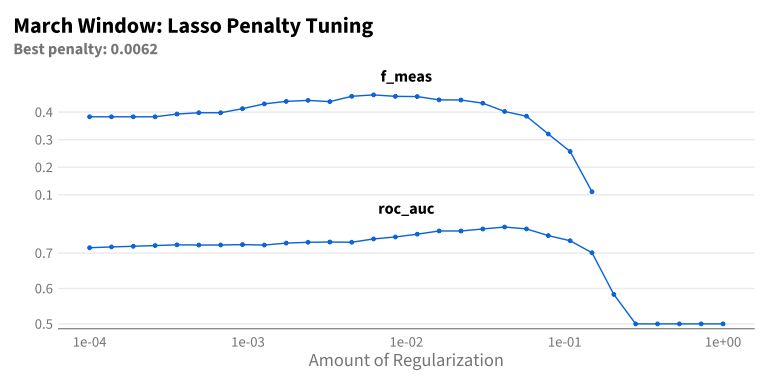
11.12.3 Lasso Tuning Plot

Code
autoplot(lasso_tune_mar) +
    labs(
        title = "March Window: Lasso Penalty Tuning",
        subtitle = paste0("Best penalty: ", round(best_lasso_penalty$penalty, 4))
    )


11.13 Appendix B: Ridge vs GLM Comparison

11.13.1 GLM Coefficient Instability

Standard logistic regression with small samples (n=42) and correlated predictors produces unstable coefficients:

Code
logreg_spec <- logistic_reg() |> set_engine("glm") |> set_mode("classification")

apr_model <- fit_classification_model(
    df_apr,
    logreg_spec,
    exclude_vars = c("pub_year", APRIL_EXCLUDE_VARS, "precip_cumsum")
)

coefs_glm <- get_logreg_coefs(apr_model)

cdi_weights_glm <- coefs_glm |>
    mutate(
        weight = -estimate / sum(abs(estimate)),
        contribution_pct = abs(weight) * 100
    ) |>
    select(term, estimate, weight, contribution_pct)

cdi_weights_glm |>
    mutate(sign_ok = if_else(weight > 0, "correct", "FLIPPED")) |>
    knitr::kable(
        digits = 3,
        col.names = c("Feature", "Raw Coef", "Weight", "Contrib %", "Sign"),
        caption = "Standard logistic regression - note coefficient sign issues"
    )
Standard logistic regression - note coefficient sign issues
Feature Raw Coef Weight Contrib % Sign
vhi -1.236 0.255 25.464 correct
mixed_fcast_obsv -1.154 0.238 23.776 correct
snow_cover -1.142 0.235 23.521 correct
asi -1.118 0.230 23.033 correct
volumetric_soil_water_1m 0.204 -0.042 4.205 FLIPPED

Problem: Some coefficients have counterintuitive signs due to multicollinearity. Ridge regression resolves this by shrinking correlated coefficients toward each other.

11.13.2 Coefficient Sign Convention

With parsnip/glmnet and levels = c("yes", "no"), the model predicts P(yes) as the first level. However, glmnet internally encodes this such that negative coefficients indicate higher probability of the first level. We negate coefficients when creating CDI weights to maintain the convention: higher CDI = more drought.

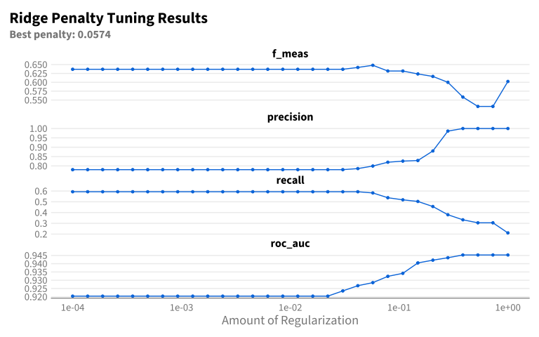
11.13.3 Ridge Tuning Plot

Code
autoplot(ridge_tune) +
    labs(
        title = "Ridge Penalty Tuning Results",
        subtitle = paste0("Best penalty: ", round(best_penalty$penalty, 4))
    )


11.14 Appendix C: Tuned Threshold Univariate Analysis

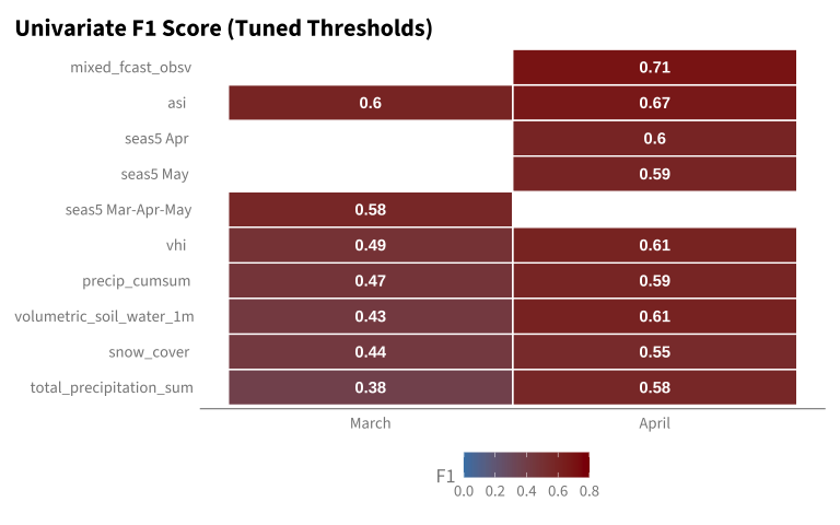
The main univariate analysis uses default P > 0.5 threshold for fair comparison. Here we show performance with thresholds tuned per predictor to maximize F1.

Code
fit_univariate_tuned <- function(data, predictor, n_boots = N_BOOTSTRAP, seed = SEED) {
    form <- as.formula(paste("drought ~", paste0("`", predictor, "`")))

    spec <- logistic_reg() |> set_engine("glm") |> set_mode("classification")
    wf <- workflow() |> add_recipe(recipe(form, data = data)) |> add_model(spec)

    set.seed(seed)
    boots <- bootstraps(data, times = n_boots, strata = drought)
    results <- fit_resamples(wf, resamples = boots,
                             control = control_resamples(save_pred = TRUE))
    preds <- collect_predictions(results)

    thresh_results <- map_dfr(seq(0.1, 0.9, by = 0.05), function(thresh) {
        pred_class <- factor(
            if_else(preds$.pred_yes > thresh, "yes", "no"),
            levels = c("yes", "no")
        )
        tibble(
            threshold = thresh,
            f1 = f_meas_vec(preds$drought, pred_class)
        )
    })

    best_thresh <- thresh_results |>
        filter(f1 == max(f1, na.rm = TRUE)) |>
        slice(1) |>
        pull(threshold)

    pred_tuned <- factor(
        if_else(preds$.pred_yes > best_thresh, "yes", "no"),
        levels = c("yes", "no")
    )

    tibble(
        predictor = predictor,
        threshold = best_thresh,
        roc_auc = roc_auc_vec(preds$drought, preds$.pred_yes),
        f_meas = f_meas_vec(preds$drought, pred_tuned),
        precision = precision_vec(preds$drought, pred_tuned),
        recall = recall_vec(preds$drought, pred_tuned)
    )
}

df_uni_apr_tuned <- map(get_predictors(df_apr), \(p) fit_univariate_tuned(df_apr, p)) |>
    list_rbind() |> mutate(window = "April")

df_uni_mar_tuned <- map(get_predictors(df_mar), \(p) fit_univariate_tuned(df_mar, p)) |>
    list_rbind() |> mutate(window = "March")

df_univariate_tuned <- bind_rows(df_uni_apr_tuned, df_uni_mar_tuned)
Code
df_univariate_tuned |>
    select(window, predictor, threshold, roc_auc, f_meas, precision, recall) |>
    arrange(window, desc(f_meas)) |>
    knitr::kable(
        digits = 3,
        caption = "Univariate predictor performance with tuned thresholds",
        col.names = c("Window", "Predictor", "Threshold", "AUC", "F1", "Precision", "Recall")
    )
Univariate predictor performance with tuned thresholds
Window Predictor Threshold AUC F1 Precision Recall
April mixed_fcast_obsv 0.30 0.874 0.705 0.612 0.832
April asi 0.30 0.872 0.674 0.674 0.674
April volumetric_soil_water_1m 0.35 0.853 0.611 0.602 0.621
April vhi 0.25 0.845 0.608 0.507 0.758
April seas5 Apr 0.30 0.774 0.597 0.507 0.726
April seas5 May 0.20 0.813 0.593 0.455 0.853
April precip_cumsum 0.40 0.815 0.590 0.690 0.516
April total_precipitation_sum 0.40 0.770 0.577 0.517 0.653
April snow_cover 0.30 0.741 0.548 0.452 0.695
March asi 0.25 0.763 0.599 0.487 0.779
March seas5 Mar-Apr-May 0.30 0.767 0.577 0.479 0.726
March vhi 0.20 0.723 0.490 0.339 0.884
March precip_cumsum 0.25 0.647 0.473 0.411 0.558
March snow_cover 0.20 0.661 0.436 0.292 0.863
March volumetric_soil_water_1m 0.20 0.667 0.433 0.311 0.716
March total_precipitation_sum 0.25 0.574 0.378 0.291 0.537
Code
df_univariate_tuned |>
    mutate(window = factor(window, levels = c("March", "April"))) |>
    ggplot(aes(x = window, y = reorder(predictor, f_meas), fill = f_meas)) +
    geom_tile(color = "white", linewidth = 0.5) +
    geom_text(aes(label = round(f_meas, 2)), color = "white", fontface = "bold") +
    scale_fill_gradient(low = "steelblue", high = "darkred", limits = c(0, 0.8)) +
    labs(
        title = "Univariate F1 Score (Tuned Thresholds)",
        x = NULL, y = NULL, fill = "F1"
    ) +
    theme(panel.grid = element_blank())

Key observation: All optimal thresholds are below 0.5 (range 0.25-0.35), confirming that the default threshold underestimates performance for imbalanced data.


11.15 Appendix D: CDI vs Predicted Probability

This appendix verifies the relationship between the manually-constructed CDI and the ridge model’s predicted probabilities, and explains when each metric is appropriate.

11.15.1 The Relationship Between CDI, Linear Predictor, and Probability

Logistic regression operates in three stages:

  1. Linear predictor = intercept + β₁x₁ + β₂x₂ + … (unbounded, can be any real number)
  2. CDI = (β₁x₁ + β₂x₂ + …) / Σ|β| (normalized linear predictor without intercept)
  3. Probability = 1 / (1 + exp(-linear_predictor)) (logistic transformation, bounded 0-1)

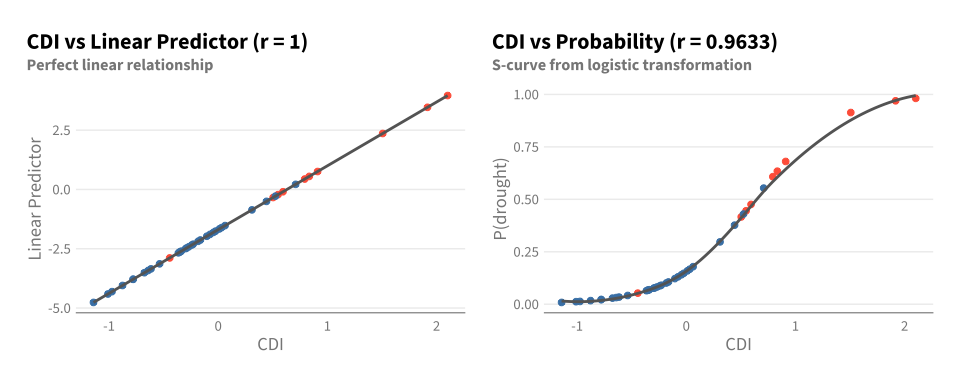
The CDI and linear predictor differ only by a shift (intercept) and scale (normalization), so they should be perfectly correlated (r = 1). The probability is a non-linear (S-curve) transformation of the linear predictor, which preserves ranking but changes distances between points.

Code
# Extract the LINEAR PREDICTOR (before logistic transformation)
# Recover from probability using inverse logistic: logit(p) = log(p/(1-p))
df_apr_probs <- df_apr_probs |>
    mutate(
        linear_predictor = log(prob_drought / (1 - prob_drought))
    )

# Correlations
cor_cdi_linear <- cor(df_apr_probs$CDI, df_apr_probs$linear_predictor)
cor_cdi_prob <- cor(df_apr_probs$CDI, df_apr_probs$prob_drought)

# Check ranking equivalence
rank_cdi <- rank(df_apr_probs$CDI)
rank_prob <- rank(df_apr_probs$prob_drought)
ranks_identical <- all(rank_cdi == rank_prob)

cat("Correlation CDI vs Linear Predictor:", round(cor_cdi_linear, 6), "\n")
Correlation CDI vs Linear Predictor: 1 
Code
cat("Correlation CDI vs Probability:", round(cor_cdi_prob, 6), "\n")
Correlation CDI vs Probability: 0.96334 
Code
cat("Rankings identical:", ranks_identical, "\n")
Rankings identical: TRUE 

As expected:

  • CDI vs Linear Predictor: r = 1 (perfect linear relationship)
  • CDI vs Probability: r ≈ 0.96 (S-curve introduces non-linearity)
  • Rankings identical: TRUE (same years would trigger at any percentile threshold)

11.15.2 Visual Verification

Code
library(patchwork)

p1 <- ggplot(df_apr_probs, aes(x = CDI, y = linear_predictor)) +
    geom_point(aes(color = drought), size = 2) +
    geom_smooth(method = "lm", se = FALSE, color = "gray40") +
    scale_color_manual(values = c("yes" = "tomato", "no" = "steelblue")) +
    labs(
        title = paste0("CDI vs Linear Predictor (r = ", round(cor_cdi_linear, 4), ")"),
        subtitle = "Perfect linear relationship",
        x = "CDI", y = "Linear Predictor"
    ) +
    theme(legend.position = "none")

p2 <- ggplot(df_apr_probs, aes(x = CDI, y = prob_drought)) +
    geom_point(aes(color = drought), size = 2) +
    geom_smooth(method = "loess", se = FALSE, color = "gray40") +
    scale_color_manual(values = c("yes" = "tomato", "no" = "steelblue")) +
    labs(
        title = paste0("CDI vs Probability (r = ", round(cor_cdi_prob, 4), ")"),
        subtitle = "S-curve from logistic transformation",
        x = "CDI", y = "P(drought)"
    ) +
    theme(legend.position = "none")

p1 + p2

The left panel shows perfect linearity between CDI and the linear predictor. The right panel shows the characteristic S-curve of the logistic transformation, which compresses extreme values toward 0 and 1.

11.15.3 Time Series Comparison

Code
# Rescale probability to same range as CDI for visual comparison
cdi_range <- range(df_apr_probs$CDI)
prob_rescaled <- scales::rescale(df_apr_probs$prob_drought, to = cdi_range)

df_comparison <- df_apr_probs |>
    mutate(
        year = pub_year,
        prob_rescaled = prob_rescaled
    )

ggplot(df_comparison, aes(x = year)) +
    geom_line(aes(y = CDI, color = "CDI"), linewidth = 1) +
    geom_line(aes(y = prob_rescaled, color = "P(drought) rescaled"),
              linewidth = 1, linetype = "dashed") +
    geom_point(aes(y = CDI, shape = drought), size = 2.5) +
    scale_color_manual(values = c("CDI" = "black", "P(drought) rescaled" = "darkred")) +
    scale_shape_manual(values = c("yes" = 16, "no" = 1),
                       labels = c("yes" = "Drought", "no" = "No drought")) +
    labs(
        title = "Time Series: CDI vs Predicted Probability",
        subtitle = "Probability rescaled to CDI range; divergence shows logistic non-linearity",
        x = "Year", y = "CDI scale",
        color = "Metric", shape = "Actual"
    )

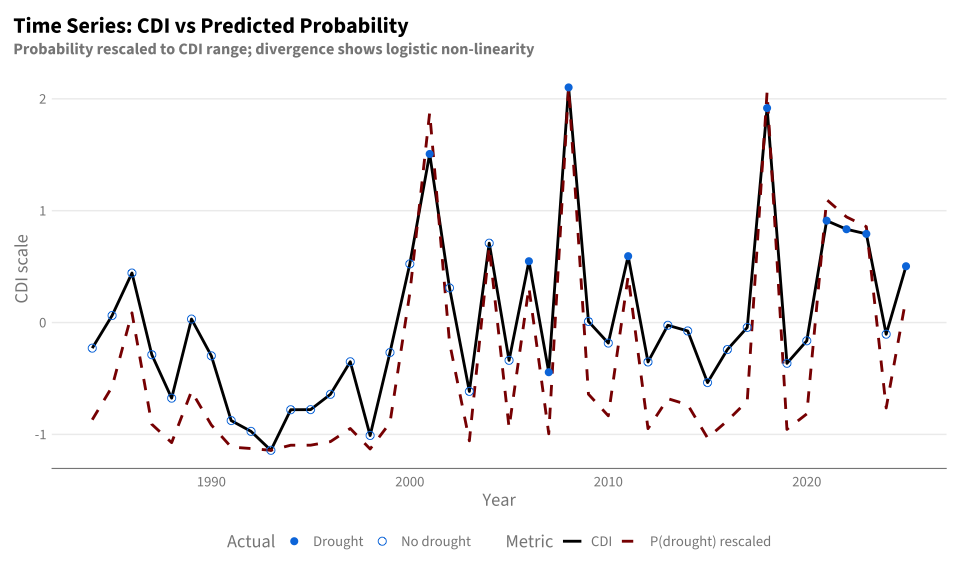
The lines track closely but diverge slightly at extreme values (e.g., peaks around 2000, 2008, 2018) where the logistic transformation compresses the scale.

11.15.4 When to Use CDI vs Probability

Use CDI when:

  • Setting percentile-based thresholds (e.g., RP=4 triggers at 75th percentile)
  • Communicating drought severity on an interpretable scale
  • Rankings and relative ordering are what matter
  • Operational simplicity is valued (CDI relates directly to input z-scores)

Use probability when:

  • Communicating risk as a percentage (“65% chance of drought this year”)
  • Decision-making with explicit cost-benefit analysis
  • Combining forecasts from multiple models (probabilities are on a standard scale)
  • Calibration matters (if verified)

11.15.5 Probability Interpretation in This Model

The predicted probability has a specific meaning: P(drought) = probability that end-of-season ASI will exceed the 4-year return period threshold, given the early-season indicator values.

This is a meaningful quantity, but:

  1. We use F1-optimized thresholds - The threshold is tuned to maximize classification performance, then expressed as an equivalent CDI value
  2. CDI is more interpretable - “CDI = 1.5” relates to input z-scores; “P = 0.72” requires calibration context
NoteSummary

The CDI is mathematically equivalent to the ridge model’s linear predictor (r = 1) and produces identical year rankings as the predicted probability. We tune the probability threshold to maximize F1, then derive the equivalent CDI cutoff — both produce identical trigger decisions. The F1-optimized threshold corresponds to approximately RP 3.9 (close to the policy target of RP 4). CDI is preferred operationally for its interpretability; probability would be appropriate if partners requested probabilistic risk communication.


11.16 Appendix F: Including Cumulative Precipitation

The 2025 trigger included cumulative precipitation (precip_cumsum) as one of the six CDI components. In the main 2026 model above, we excluded it due to collinearity concerns with other precipitation-related variables. This appendix tests whether including it improves model performance.

11.16.1 Model with All 2025 Variables

We fit a ridge model including precip_cumsum alongside the other indicators, matching the 2025 variable set (except using the composite mixed_fcast_obsv instead of individual forecast months).

Code
# Ridge model INCLUDING precip_cumsum
ridge_recipe_precip <- recipe(drought ~ ., data = df_apr) |>
    step_rm(all_of(c("pub_year", APRIL_EXCLUDE_VARS))) |>  # Note: NOT removing precip_cumsum
    step_zv(all_predictors())

ridge_wf_precip <- workflow() |>
    add_recipe(ridge_recipe_precip) |>
    add_model(ridge_spec)

# Bootstrap resampling with penalty tuning
set.seed(SEED)
ridge_boots_precip <- bootstraps(df_apr, times = N_BOOTSTRAP, strata = drought)

ridge_tune_precip <- tune_grid(
    ridge_wf_precip,
    resamples = ridge_boots_precip,
    grid = penalty_grid,
    metrics = metric_set(roc_auc, f_meas, precision, recall),
    control = control_grid(save_pred = TRUE)
)

# Select best penalty
best_penalty_precip <- select_best(ridge_tune_precip, metric = "f_meas")
final_ridge_fit_precip <- fit(
    ridge_wf_precip |> finalize_workflow(best_penalty_precip),
    data = df_apr
)

# Extract coefficients
coefs_ridge_precip <- final_ridge_fit_precip |>
    extract_fit_parsnip() |>
    tidy() |>
    filter(term != "(Intercept)")

cdi_weights_precip <- coefs_ridge_precip |>
    mutate(
        weight = -estimate / sum(abs(estimate)),
        contribution_pct = abs(weight) * 100
    ) |>
    arrange(desc(contribution_pct)) |>
    select(term, estimate, weight, contribution_pct)

11.16.2 CDI Weights with Cumulative Precipitation

Code
cdi_weights_precip |>
    knitr::kable(
        digits = 3,
        col.names = c("Indicator", "Ridge Coef", "CDI Weight", "Contribution %"),
        caption = "CDI weights including cumulative precipitation"
    )
CDI weights including cumulative precipitation
Indicator Ridge Coef CDI Weight Contribution %
mixed_fcast_obsv -0.737 0.274 27.361
asi -0.551 0.205 20.455
snow_cover -0.550 0.204 20.417
vhi -0.515 0.191 19.138
volumetric_soil_water_1m -0.317 0.118 11.786
precip_cumsum -0.023 0.008 0.844

11.16.3 LOOCV Performance Comparison

Code
# LOOCV for model with precip_cumsum
loocv_precip_results <- map_dfr(1:nrow(df_apr), function(i) {
    train <- df_apr[-i, ]
    test <- df_apr[i, ]

    rec <- recipe(drought ~ ., data = train) |>
        step_rm(all_of(c("pub_year", APRIL_EXCLUDE_VARS))) |>
        step_zv(all_predictors())

    spec <- logistic_reg(penalty = best_penalty_precip$penalty, mixture = 0) |>
        set_engine("glmnet") |>
        set_mode("classification")

    wf <- workflow() |>
        add_recipe(rec) |>
        add_model(spec)

    fit_result <- fit(wf, data = train)

    # Get probability for ROC AUC
    prob <- predict(fit_result, test, type = "prob")$.pred_yes

    # CDI-based trigger
    coefs <- fit_result |>
        extract_fit_parsnip() |>
        tidy() |>
        filter(term != "(Intercept)") |>
        mutate(weight = -estimate / sum(abs(estimate)))

    train_cdi <- rep(0, nrow(train))
    for (j in seq_len(nrow(coefs))) {
        feat <- coefs$term[j]
        w <- coefs$weight[j]
        if (feat %in% colnames(train)) {
            train_cdi <- train_cdi + w * train[[feat]]
        }
    }
    train_rp <- rp_empirical(train_cdi, direction = "-1")
    threshold <- min(train_cdi[train_rp >= RP_THRESHOLD])

    test_cdi <- 0
    for (j in seq_len(nrow(coefs))) {
        feat <- coefs$term[j]
        w <- coefs$weight[j]
        if (feat %in% colnames(test)) {
            test_cdi <- test_cdi + w * test[[feat]]
        }
    }

    tibble(
        year = test$pub_year,
        actual = test$drought,
        prob = prob,
        predicted = if_else(test_cdi >= threshold, "yes", "no")
    )
})

# Confusion matrix
loocv_precip_conf <- table(
    Predicted = factor(loocv_precip_results$predicted, levels = c("yes", "no")),
    Actual = factor(loocv_precip_results$actual, levels = c("yes", "no"))
)

tp_precip <- loocv_precip_conf["yes", "yes"]
fp_precip <- loocv_precip_conf["yes", "no"]
fn_precip <- loocv_precip_conf["no", "yes"]
Code
# Comparison table
tibble(
    Model = c("Without precip_cumsum (main)", "With precip_cumsum"),
    `N Features` = c(nrow(cdi_weights), nrow(cdi_weights_precip)),
    `ROC AUC` = c(
        round(yardstick::roc_auc_vec(loocv_composite_probs$actual, loocv_composite_probs$prob), 3),
        round(yardstick::roc_auc_vec(loocv_precip_results$actual, loocv_precip_results$prob), 3)
    ),
    Precision = c(
        round(tp_ridge_loo / (tp_ridge_loo + fp_ridge_loo), 3),
        round(tp_precip / (tp_precip + fp_precip), 3)
    ),
    Recall = c(
        round(tp_ridge_loo / (tp_ridge_loo + fn_ridge_loo), 3),
        round(tp_precip / (tp_precip + fn_precip), 3)
    ),
    F1 = c(
        round(2 * tp_ridge_loo / (2 * tp_ridge_loo + fp_ridge_loo + fn_ridge_loo), 3),
        round(2 * tp_precip / (2 * tp_precip + fp_precip + fn_precip), 3)
    )
) |>
    knitr::kable(caption = "LOOCV comparison: With vs without cumulative precipitation")
LOOCV comparison: With vs without cumulative precipitation
Model N Features ROC AUC Precision Recall F1
Without precip_cumsum (main) 5 0.869 0.727 0.8 0.762
With precip_cumsum 6 0.862 0.700 0.7 0.700

11.16.4 LOOCV Confusion Matrices

Code
cat("Without precip_cumsum (main model):\n")
Without precip_cumsum (main model):
Code
loocv_ridge_conf |>
    as.data.frame.matrix() |>
    knitr::kable()
yes no
yes 8 3
no 2 29
Code
cat("\nWith precip_cumsum:\n")

With precip_cumsum:
Code
loocv_precip_conf |>
    as.data.frame.matrix() |>
    knitr::kable()
yes no
yes 7 3
no 3 29

11.16.5 Weight Comparison

How does including cumulative precipitation change the weights assigned to other components?

Code
# Combine weights for comparison
df_weight_compare <- bind_rows(
    cdi_weights |> mutate(model = "Without precip_cumsum"),
    cdi_weights_precip |> mutate(model = "With precip_cumsum")
) |>
    select(model, term, weight, contribution_pct)

df_weight_compare |>
    ggplot(aes(x = reorder(term, contribution_pct), y = contribution_pct, fill = model)) +
    geom_col(position = position_dodge(width = 0.8), width = 0.7) +
    geom_text(
        aes(label = paste0(round(contribution_pct, 0), "%")),
        position = position_dodge(width = 0.8),
        hjust = -0.1, size = 3
    ) +
    coord_flip() +
    scale_fill_manual(values = c("Without precip_cumsum" = "steelblue",
                                  "With precip_cumsum" = "tomato")) +
    scale_y_continuous(limits = c(0, 35), expand = c(0, 0)) +
    labs(
        title = "CDI Component Weights: With vs Without Cumulative Precipitation",
        x = NULL, y = "Contribution (%)", fill = "Model"
    ) +
    theme(legend.position = "top")

NoteFinding

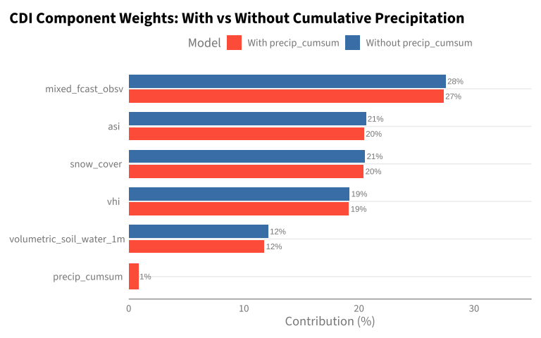
Including cumulative precipitation (precip_cumsum) in the April CDI model produces similar LOOCV performance to the main model without it. The variable receives a weight of approximately 1%, redistributing weight away from the other indicators.

The similar performance suggests that cumulative precipitation provides partially redundant information — its signal is already captured by other indicators (soil moisture, the mixed forecast/observation composite). For operational simplicity, the main 5-component model is preferred.

11.16.6 Year-by-Year Comparison

Do the two models trigger on the same years?

Code
# Merge predictions
df_year_compare <- loocv_ridge_results |>
    select(year, actual, predicted_main = predicted) |>
    left_join(
        loocv_precip_results |> select(year, predicted_precip = predicted),
        by = "year"
    ) |>
    mutate(
        agree = predicted_main == predicted_precip,
        both_correct = predicted_main == actual & predicted_precip == actual,
        main_only_correct = predicted_main == actual & predicted_precip != actual,
        precip_only_correct = predicted_precip == actual & predicted_main != actual
    )

# Summary
cat("Agreement between models:\n")
Agreement between models:
Code
cat("  Same prediction:", sum(df_year_compare$agree), "of", nrow(df_year_compare), "years\n")
  Same prediction: 41 of 42 years
Code
cat("  Disagreements:", sum(!df_year_compare$agree), "years\n\n")
  Disagreements: 1 years
Code
# Show disagreements if any
if (sum(!df_year_compare$agree) > 0) {
    cat("Years where models disagree:\n")
    df_year_compare |>
        filter(!agree) |>
        select(year, actual, predicted_main, predicted_precip) |>
        knitr::kable(col.names = c("Year", "Actual", "Main Model", "With Precip"))
}
Years where models disagree:
Year Actual Main Model With Precip
2006 yes yes no