13  CERF Allocation Alignment

13.1 Introduction

This chapter evaluates how well the proposed trigger signals align with historical CERF Rapid Response drought allocations for Afghanistan. CERF Rapid Response allocations represent an independent, external validation of drought severity — they reflect the humanitarian community’s real-time assessment that conditions warranted emergency funding.

We filter to Rapid Response allocations only (excluding Underfunded Emergencies), as these represent the acute drought response most analogous to anticipatory action triggers. We treat CERF Rapid Response allocation as the outcome variable and ask: if we had applied our CDI or SEAS5 triggers historically, how often would they have correctly predicted a CERF allocation year?

Code
box::use(
    dplyr[...],
    tidyr[...],
    ggplot2[...],
    gghdx[...],
    cumulus[...],
    purrr[...],
    glue[glue],
    tibble[tibble],
    janitor[clean_names],
    lubridate[year, as_date],
    .. / R / utils[rp_empirical]
)

library(tidymodels)
library(gt)
gghdx()
Code
RP_THRESHOLD <- 4
SEED <- 42
N_BOOTSTRAP <- 30

FEATURE_PATHS <- list(
    march = "ds-aa-afg-drought/processed/vector/2026_mar_pub_feature_set_v1.parquet",
    april = "ds-aa-afg-drought/processed/vector/2026_april_pub_feature_set_v1.parquet"
)

APRIL_EXCLUDE_VARS <- c("total_precipitation_sum", "seas5 Apr", "seas5 May")

13.2 Data

Code
# Load feature sets
df_mar_raw <- blob_read(name = FEATURE_PATHS$march, container = "projects")
df_apr_raw <- blob_read(name = FEATURE_PATHS$april, container = "projects")

# Prepare modeling data
prepare_model_data <- function(df, rp_threshold = RP_THRESHOLD) {
    df |>
        filter(!is.na(outcome_asi_zscore)) |>
        arrange(desc(outcome_asi_zscore)) |>
        mutate(
            rank = row_number(),
            q_rank = rank / (n() + 1),
            rp_emp = 1 / q_rank,
            drought = factor(
                if_else(rp_emp >= rp_threshold, "yes", "no"),
                levels = c("yes", "no")
            )
        ) |>
        select(-outcome_asi_zscore, -rank, -q_rank, -rp_emp,
               -starts_with("adm0_name"), -pub_date, -timestep)
}

df_mar <- prepare_model_data(df_mar_raw)
df_apr <- prepare_model_data(df_apr_raw)
Code
ridge_spec <- logistic_reg(penalty = tune(), mixture = 0) |>
    set_engine("glmnet") |>
    set_mode("classification")

ridge_recipe <- recipe(drought ~ ., data = df_apr) |>
    step_rm(all_of(c("pub_year", APRIL_EXCLUDE_VARS, "precip_cumsum"))) |>
    step_zv(all_predictors())

ridge_wf <- workflow() |>
    add_recipe(ridge_recipe) |>
    add_model(ridge_spec)

set.seed(SEED)
ridge_boots <- bootstraps(df_apr, times = N_BOOTSTRAP, strata = drought)
penalty_grid <- grid_regular(penalty(range = c(-4, 0)), levels = 30)

ridge_tune <- tune_grid(
    ridge_wf,
    resamples = ridge_boots,
    grid = penalty_grid,
    metrics = metric_set(roc_auc, f_meas),
    control = control_grid(save_pred = TRUE)
)

best_penalty <- select_best(ridge_tune, metric = "f_meas")
final_ridge_fit <- fit(finalize_workflow(ridge_wf, best_penalty), data = df_apr)

coefs_ridge <- final_ridge_fit |>
    extract_fit_parsnip() |>
    tidy() |>
    filter(term != "(Intercept)")

cdi_weights <- coefs_ridge |>
    mutate(
        weight = -estimate / sum(abs(estimate)),
        contribution_pct = abs(weight) * 100
    ) |>
    arrange(desc(contribution_pct)) |>
    select(term, estimate, weight, contribution_pct)

# F1-optimized probability threshold → CDI threshold (same derivation as ch12)
prob_drought <- predict(final_ridge_fit, df_apr, type = "prob")$.pred_yes

thresholds <- seq(0.1, 0.9, by = 0.05)
best_prob_threshold <- map_dfr(thresholds, function(thresh) {
    pred <- factor(if_else(prob_drought > thresh, "yes", "no"), levels = c("yes", "no"))
    tibble(threshold = thresh, f1 = yardstick::f_meas_vec(df_apr$drought, pred))
}) |>
    filter(f1 == max(f1, na.rm = TRUE)) |>
    slice(1) |>
    pull(threshold)
Code
df_cerf <- blob_read("ds-aa-afg-drought/raw/vector/afg_drought_cerf_allocations.xlsx") |>
    clean_names() |>
    mutate(allocation_date = as_date(allocation_date)) |>
    filter(window == "Rapid Response")

df_cerf_yr <- df_cerf |>
    group_by(yr = year(allocation_date)) |>
    summarise(n_allocations = n()) |>
    # 2025 CERF Rapid Response allocation occurred but is not yet in the dataset
    bind_rows(tibble(yr = 2025, n_allocations = 1)) |>
    complete(yr = 2006:2025, fill = list(n_allocations = 0)) |>
    mutate(cerf = factor(if_else(n_allocations > 0, "yes", "no"), levels = c("yes", "no")))
Code
calc_cdi <- function(data, weights_df) {
    cdi <- rep(0, nrow(data))
    for (i in seq_len(nrow(weights_df))) {
        feat <- weights_df$term[i]
        w <- weights_df$weight[i]
        if (feat %in% colnames(data)) {
            cdi <- cdi + w * data[[feat]]
        }
    }
    cdi
}

df_historical <- tibble(
    year = df_apr$pub_year,
    drought_actual = df_apr$drought,
    cdi = calc_cdi(df_apr, cdi_weights),
    prob_drought = prob_drought,
    seas5_mam = df_mar$`seas5 Mar-Apr-May`
) |>
    mutate(
        cdi_rp = rp_empirical(cdi, direction = "-1"),
        seas5_rp = rp_empirical(seas5_mam, direction = "-1")
    )

# CDI threshold from F1-optimized probability (consistent with ch12)
cdi_threshold <- min(df_historical$cdi[df_historical$prob_drought > best_prob_threshold])

# Join with CERF data — restrict to CERF coverage period (2006–2024)
df_cerf_analysis <- df_historical |>
    inner_join(df_cerf_yr, by = c("year" = "yr"))

CERF allocation years: 2006, 2008, 2018, 2021, 2025.

Analysis period: 2006–2025 (20 years), of which 5 had CERF drought allocations.

13.3 ROC-AUC: Continuous Signal Quality

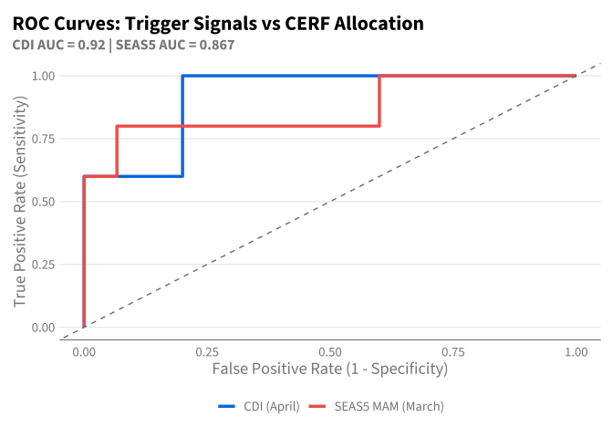
Before examining thresholds, we evaluate how well the continuous CDI and SEAS5 scores discriminate CERF allocation years from non-allocation years. ROC-AUC is threshold-independent and measures overall ranking quality.

Code
roc_cdi <- yardstick::roc_auc_vec(
    df_cerf_analysis$cerf,
    df_cerf_analysis$cdi
)

roc_seas5 <- yardstick::roc_auc_vec(
    df_cerf_analysis$cerf,
    df_cerf_analysis$seas5_mam
)

tibble(
    Signal = c("CDI (April)", "SEAS5 MAM (March)"),
    `ROC-AUC` = c(roc_cdi, roc_seas5)
) |>
    gt() |>
    tab_header(
        title = "ROC-AUC: Continuous Signal vs CERF Allocation",
        subtitle = glue("{min(df_cerf_analysis$year)}\u2013{max(df_cerf_analysis$year)}")
    ) |>
    fmt_number(columns = `ROC-AUC`, decimals = 3)
ROC-AUC: Continuous Signal vs CERF Allocation
2006–2025
Signal ROC-AUC
CDI (April) 0.920
SEAS5 MAM (March) 0.867
Code
roc_data_cdi <- yardstick::roc_curve(
    df_cerf_analysis |> mutate(cerf = factor(cerf, levels = c("yes", "no"))),
    cerf,
    cdi
) |> mutate(signal = "CDI (April)")

roc_data_seas5 <- yardstick::roc_curve(
    df_cerf_analysis |> mutate(cerf = factor(cerf, levels = c("yes", "no"))),
    cerf,
    seas5_mam
) |> mutate(signal = "SEAS5 MAM (March)")

bind_rows(roc_data_cdi, roc_data_seas5) |>
    ggplot(aes(x = 1 - specificity, y = sensitivity, color = signal)) +
    geom_path(linewidth = 1.2) +
    geom_abline(linetype = "dashed", color = "grey50") +
    scale_color_manual(values = c(
        "CDI (April)" = hdx_hex("sapphire-hdx"),
        "SEAS5 MAM (March)" = hdx_hex("tomato-hdx")
    )) +
    labs(
        title = "ROC Curves: Trigger Signals vs CERF Allocation",
        subtitle = glue("CDI AUC = {round(roc_cdi, 3)} | SEAS5 AUC = {round(roc_seas5, 3)}"),
        x = "False Positive Rate (1 - Specificity)",
        y = "True Positive Rate (Sensitivity)",
        color = NULL
    )

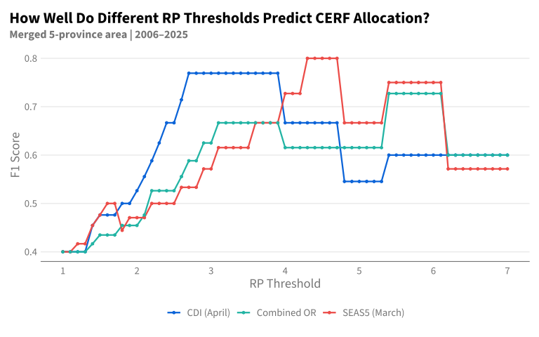
13.4 F1 by RP Threshold

For each RP threshold, we flag years where CDI or SEAS5 exceeds the threshold and compute classification metrics against CERF allocation.

Code
df_f1_by_rp <- map_dfr(seq(1, 7, by = 0.1), function(rp) {
    cdi_flag <- factor(
        if_else(df_cerf_analysis$cdi_rp >= rp, "yes", "no"),
        levels = c("yes", "no")
    )
    seas5_flag <- factor(
        if_else(df_cerf_analysis$seas5_rp >= rp, "yes", "no"),
        levels = c("yes", "no")
    )
    combined_flag <- factor(
        if_else(df_cerf_analysis$cdi_rp >= rp | df_cerf_analysis$seas5_rp >= rp, "yes", "no"),
        levels = c("yes", "no")
    )

    cerf_truth <- df_cerf_analysis$cerf

    calc_metrics <- function(pred, label) {
        tibble(
            signal = label,
            rp = rp,
            f1 = yardstick::f_meas_vec(cerf_truth, pred),
            precision = yardstick::precision_vec(cerf_truth, pred),
            recall = yardstick::recall_vec(cerf_truth, pred)
        )
    }

    bind_rows(
        calc_metrics(cdi_flag, "CDI (April)"),
        calc_metrics(seas5_flag, "SEAS5 (March)"),
        calc_metrics(combined_flag, "Combined OR")
    )
})
Code
df_f1_by_rp |>
    ggplot(aes(x = rp, y = f1, color = signal)) +
    geom_line(linewidth = 0.8) +
    geom_point(size = 1) +
    scale_x_continuous(breaks = 1:7) +
    scale_color_manual(values = c(
        "CDI (April)" = hdx_hex("sapphire-hdx"),
        "SEAS5 (March)" = hdx_hex("tomato-hdx"),
        "Combined OR" = hdx_hex("mint-hdx")
    )) +
    labs(
        title = "How Well Do Different RP Thresholds Predict CERF Allocation?",
        subtitle = glue("Merged 5-province area | {min(df_cerf_analysis$year)}\u2013{max(df_cerf_analysis$year)}"),
        x = "RP Threshold",
        y = "F1 Score",
        color = NULL
    )

Code
df_f1_by_rp |>
    filter(rp %in% 2:6) |>
    mutate(across(c(f1, precision, recall), \(x) round(x, 3))) |>
    pivot_wider(
        names_from = signal,
        values_from = c(f1, precision, recall),
        names_glue = "{signal}_{.value}"
    ) |>
    select(rp, starts_with("CDI"), starts_with("SEAS5"), starts_with("Combined")) |>
    gt() |>
    tab_header(
        title = "Classification Metrics by RP Threshold",
        subtitle = "CERF allocation as outcome"
    ) |>
    tab_spanner(label = "CDI (April)", columns = starts_with("CDI")) |>
    tab_spanner(label = "SEAS5 (March)", columns = starts_with("SEAS5")) |>
    tab_spanner(label = "Combined OR", columns = starts_with("Combined")) |>
    cols_label(
        rp = "RP",
        `CDI (April)_f1` = "F1",
        `CDI (April)_precision` = "Prec",
        `CDI (April)_recall` = "Rec",
        `SEAS5 (March)_f1` = "F1",
        `SEAS5 (March)_precision` = "Prec",
        `SEAS5 (March)_recall` = "Rec",
        `Combined OR_f1` = "F1",
        `Combined OR_precision` = "Prec",
        `Combined OR_recall` = "Rec"
    )
Classification Metrics by RP Threshold
CERF allocation as outcome
RP CDI (April) SEAS5 (March) Combined OR
F1 Prec Rec F1 Prec Rec F1 Prec Rec
2 0.526 0.357 1.0 0.471 0.333 0.8 0.455 0.294 1.0
3 0.769 0.625 1.0 0.571 0.444 0.8 0.625 0.455 1.0
4 0.667 0.571 0.8 0.727 0.667 0.8 0.615 0.500 0.8
5 0.545 0.500 0.6 0.667 0.750 0.6 0.615 0.500 0.8
6 0.600 0.600 0.6 0.750 1.000 0.6 0.727 0.667 0.8

13.5 Asymmetric RP Threshold Heatmap

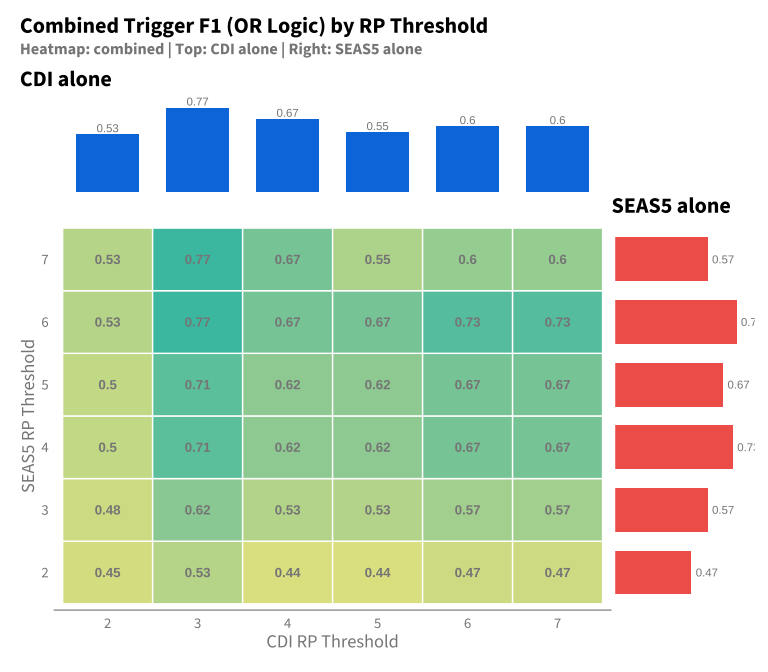
The plot above shows performance when both signals use the same RP threshold. But CDI and SEAS5 may have different optimal thresholds. The heatmap below explores all combinations, with marginal bar plots showing each signal’s standalone performance.

Code
# Compute F1 for all CDI × SEAS5 RP combinations
df_asymmetric <- expand_grid(
    cdi_rp_thresh = 2:7,
    seas5_rp_thresh = 2:7
) |>
    pmap_dfr(function(cdi_rp_thresh, seas5_rp_thresh) {
        combined_flag <- factor(
            if_else(
                df_cerf_analysis$cdi_rp >= cdi_rp_thresh |
                df_cerf_analysis$seas5_rp >= seas5_rp_thresh,
                "yes", "no"
            ),
            levels = c("yes", "no")
        )

        f1 <- yardstick::f_meas_vec(df_cerf_analysis$cerf, combined_flag)

        tibble(
            cdi_rp_thresh = cdi_rp_thresh,
            seas5_rp_thresh = seas5_rp_thresh,
            f1 = if_else(is.na(f1), 0, f1)
        )
    })

# Marginal F1 for CDI alone
df_cdi_marginal <- map_dfr(2:7, function(rp) {
    flag <- factor(
        if_else(df_cerf_analysis$cdi_rp >= rp, "yes", "no"),
        levels = c("yes", "no")
    )
    f1 <- yardstick::f_meas_vec(df_cerf_analysis$cerf, flag)
    tibble(rp = rp, f1 = if_else(is.na(f1), 0, f1))
})

# Marginal F1 for SEAS5 alone
df_seas5_marginal <- map_dfr(2:7, function(rp) {
    flag <- factor(
        if_else(df_cerf_analysis$seas5_rp >= rp, "yes", "no"),
        levels = c("yes", "no")
    )
    f1 <- yardstick::f_meas_vec(df_cerf_analysis$cerf, flag)
    tibble(rp = rp, f1 = if_else(is.na(f1), 0, f1))
})
Code
library(patchwork)

# Main heatmap
p_heat <- df_asymmetric |>
    ggplot(aes(x = factor(cdi_rp_thresh), y = factor(seas5_rp_thresh), fill = f1)) +
    geom_tile(color = "white", linewidth = 0.5) +
    geom_text(aes(label = round(f1, 2)), size = 3.5, fontface = "bold") +
    scale_fill_gradient2(
        low = "white", mid = "khaki", high = hdx_hex("mint-hdx"),
        midpoint = 0.4,
        limits = c(0, max(df_asymmetric$f1)),
        name = "F1"
    ) +
    labs(x = "CDI RP Threshold", y = "SEAS5 RP Threshold") +
    theme(
        panel.grid = element_blank(),
        legend.position = "none",
        plot.margin = margin(0, 0, 5, 5)
    )

# Top marginal bar (CDI)
p_top <- df_cdi_marginal |>
    ggplot(aes(x = factor(rp), y = f1)) +
    geom_col(fill = hdx_hex("sapphire-hdx"), width = 0.7) +
    geom_text(aes(label = round(f1, 2)), vjust = -0.3, size = 3) +
    scale_y_continuous(limits = c(0, max(df_cdi_marginal$f1) * 1.15), expand = c(0, 0)) +
    labs(x = NULL, y = NULL, title = "CDI alone") +
    theme(
        axis.text.x = element_blank(),
        axis.ticks.x = element_blank(),
        axis.text.y = element_blank(),
        axis.ticks.y = element_blank(),
        axis.line = element_blank(),
        panel.grid = element_blank(),
        plot.margin = margin(0, 0, -10, 0)
    )

# Right marginal bar (SEAS5)
p_right <- df_seas5_marginal |>
    ggplot(aes(x = f1, y = factor(rp))) +
    geom_col(fill = hdx_hex("tomato-hdx"), width = 0.7) +
    geom_text(aes(label = round(f1, 2)), hjust = -0.2, size = 3) +
    scale_x_continuous(limits = c(0, max(df_seas5_marginal$f1) * 1.15), expand = c(0, 0)) +
    labs(x = NULL, y = NULL, title = "SEAS5 alone") +
    theme(
        axis.text.x = element_blank(),
        axis.ticks.x = element_blank(),
        axis.text.y = element_blank(),
        axis.ticks.y = element_blank(),
        axis.line = element_blank(),
        panel.grid = element_blank(),
        plot.margin = margin(0, 0, 0, -10)
    )

# Empty corner
p_empty <- ggplot() + theme_void()

# Combine with patchwork
(p_top + p_empty + p_heat + p_right) +
    plot_layout(
        widths = c(4, 1),
        heights = c(1, 4)
    ) +
    plot_annotation(
        title = "Combined Trigger F1 (OR Logic) by RP Threshold",
        subtitle = "Heatmap: combined | Top: CDI alone | Right: SEAS5 alone"
    )

13.5.1 Zoomed View: RP 3–5 Range

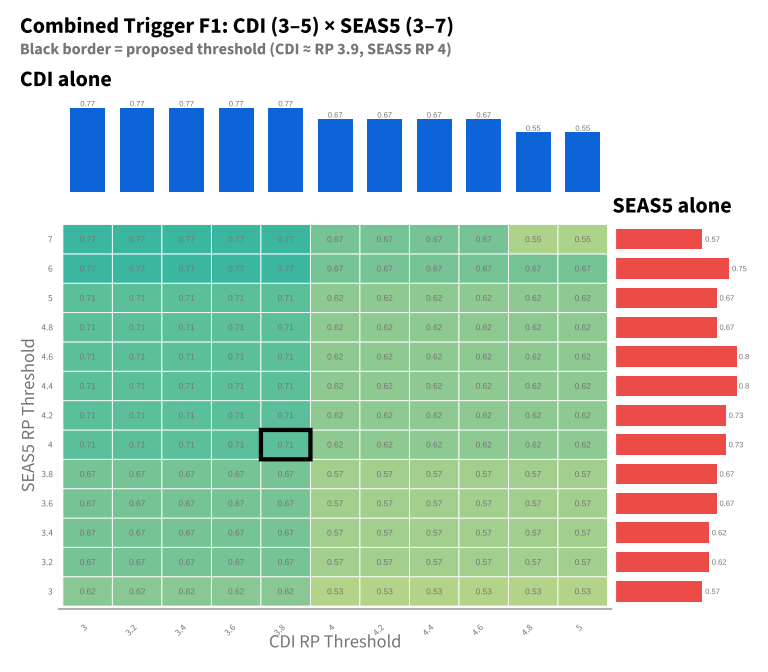
The overview heatmap uses integer RP thresholds. The zoomed view below uses 0.1 increments to show exactly where our F1-tuned threshold (~RP 3.9) sits within the optimal range.

Code
# Fine-grained RP breaks for CDI (3-5), extended range for SEAS5 (3-7)
rp_cdi_fine <- seq(3, 5, by = 0.2)
rp_seas5_fine <- c(seq(3, 5, by = 0.2), 6, 7)  # Fine 3-5, then 6, 7

# Compute our tuned threshold's equivalent RP
n_trigger_tuned <- sum(df_historical$prob_drought > best_prob_threshold)
tuned_rp <- round((nrow(df_historical) + 1) / n_trigger_tuned, 1)

df_zoom <- expand_grid(
    cdi_rp_thresh = rp_cdi_fine,
    seas5_rp_thresh = rp_seas5_fine
) |>
    pmap_dfr(function(cdi_rp_thresh, seas5_rp_thresh) {
        combined_flag <- factor(
            if_else(
                df_cerf_analysis$cdi_rp >= cdi_rp_thresh |
                df_cerf_analysis$seas5_rp >= seas5_rp_thresh,
                "yes", "no"
            ),
            levels = c("yes", "no")
        )
        f1 <- yardstick::f_meas_vec(df_cerf_analysis$cerf, combined_flag)
        tibble(
            cdi_rp_thresh = cdi_rp_thresh,
            seas5_rp_thresh = seas5_rp_thresh,
            f1 = if_else(is.na(f1), 0, f1)
        )
    })

# Marginal F1 for CDI alone (zoomed range)
df_cdi_zoom <- map_dfr(rp_cdi_fine, function(rp) {
    flag <- factor(
        if_else(df_cerf_analysis$cdi_rp >= rp, "yes", "no"),
        levels = c("yes", "no")
    )
    f1 <- yardstick::f_meas_vec(df_cerf_analysis$cerf, flag)
    tibble(rp = rp, f1 = if_else(is.na(f1), 0, f1))
})

# Marginal F1 for SEAS5 alone (extended range to 7)
df_seas5_zoom <- map_dfr(rp_seas5_fine, function(rp) {
    flag <- factor(
        if_else(df_cerf_analysis$seas5_rp >= rp, "yes", "no"),
        levels = c("yes", "no")
    )
    f1 <- yardstick::f_meas_vec(df_cerf_analysis$cerf, flag)
    tibble(rp = rp, f1 = if_else(is.na(f1), 0, f1))
})

# Find position of our tuned threshold (snap to nearest grid point)
tuned_cdi_snap <- rp_cdi_fine[which.min(abs(rp_cdi_fine - tuned_rp))]

# Main heatmap
p_heat_zoom <- df_zoom |>
    ggplot(aes(x = factor(cdi_rp_thresh), y = factor(seas5_rp_thresh), fill = f1)) +
    geom_tile(color = "white", linewidth = 0.3) +
    geom_text(aes(label = round(f1, 2)), size = 2.2) +
    # Highlight our tuned threshold
    annotate("rect",
             xmin = which(rp_cdi_fine == tuned_cdi_snap) - 0.5,
             xmax = which(rp_cdi_fine == tuned_cdi_snap) + 0.5,
             ymin = which(rp_seas5_fine == 4) - 0.5,
             ymax = which(rp_seas5_fine == 4) + 0.5,
             fill = NA, color = "black", linewidth = 1.5) +
    scale_fill_gradient2(
        low = "white", mid = "khaki", high = hdx_hex("mint-hdx"),
        midpoint = 0.4,
        limits = c(0, max(df_zoom$f1)),
        name = "F1"
    ) +
    labs(x = "CDI RP Threshold", y = "SEAS5 RP Threshold") +
    theme(
        panel.grid = element_blank(),
        legend.position = "none",
        plot.margin = margin(0, 0, 5, 5),
        axis.text.x = element_text(size = 7, angle = 45, hjust = 1),
        axis.text.y = element_text(size = 7)
    )

# Top marginal bar (CDI)
p_top_zoom <- df_cdi_zoom |>
    ggplot(aes(x = factor(rp), y = f1)) +
    geom_col(fill = hdx_hex("sapphire-hdx"), width = 0.7) +
    geom_text(aes(label = round(f1, 2)), vjust = -0.3, size = 2) +
    scale_y_continuous(limits = c(0, max(df_cdi_zoom$f1) * 1.15), expand = c(0, 0)) +
    labs(x = NULL, y = NULL, title = "CDI alone") +
    theme(
        axis.text.x = element_blank(),
        axis.ticks.x = element_blank(),
        axis.text.y = element_blank(),
        axis.ticks.y = element_blank(),
        axis.line = element_blank(),
        panel.grid = element_blank(),
        plot.margin = margin(0, 0, -10, 0)
    )

# Right marginal bar (SEAS5)
p_right_zoom <- df_seas5_zoom |>
    ggplot(aes(x = f1, y = factor(rp))) +
    geom_col(fill = hdx_hex("tomato-hdx"), width = 0.7) +
    geom_text(aes(label = round(f1, 2)), hjust = -0.2, size = 2) +
    scale_x_continuous(limits = c(0, max(df_seas5_zoom$f1) * 1.15), expand = c(0, 0)) +
    labs(x = NULL, y = NULL, title = "SEAS5 alone") +
    theme(
        axis.text.x = element_blank(),
        axis.ticks.x = element_blank(),
        axis.text.y = element_blank(),
        axis.ticks.y = element_blank(),
        axis.line = element_blank(),
        panel.grid = element_blank(),
        plot.margin = margin(0, 0, 0, -10)
    )

# Empty corner
p_empty_zoom <- ggplot() + theme_void()

# Combine with patchwork
(p_top_zoom + p_empty_zoom + p_heat_zoom + p_right_zoom) +
    plot_layout(
        widths = c(4, 1),
        heights = c(1, 4)
    ) +
    plot_annotation(
        title = "Combined Trigger F1: CDI (3–5) × SEAS5 (3–7)",
        subtitle = glue("Black border = proposed threshold (CDI ≈ RP {tuned_rp}, SEAS5 RP 4)")
    )
NoteInterpretation

CERF alignment shows a plateau in the RP 3–5 range — lowering the threshold doesn’t improve performance (the same years trigger within the CERF period), and raising it only marginally affects F1 until you start missing CERF years at RP ≥ 5. This means CERF performance alone doesn’t determine the optimal threshold.

The early:false ratio (see previous chapter) breaks the tie: within the CERF-optimal plateau, SEAS5 RP ≥ 4 maximizes early warning value (6/10 droughts get March warning) while minimizing false early alerts (4 over 42 years, ratio 1.5:1). Lowering to RP 3 adds false alerts without improving CERF alignment; raising to RP 5 loses recent droughts (2021, 2023) without removing false positives.

Bottom line: RP ~4 sits in the sweet spot — optimal for CERF alignment AND best early:false ratio for anticipatory action.

13.6 Year-by-Year Alignment

Code
df_cerf_analysis |>
    mutate(
        cdi_trig = if_else(cdi >= cdi_threshold, "yes", "no"),
        seas5_rp4 = if_else(seas5_rp >= 4, "yes", "no"),
        combined = if_else(cdi >= cdi_threshold | seas5_rp >= 4, "yes", "no")
    ) |>
    select(year, cerf, drought_actual, cdi_trig, seas5_rp4, combined) |>
    arrange(desc(year)) |>
    rename(
        Year = year,
        CERF = cerf,
        `ASI Drought` = drought_actual,
        CDI = cdi_trig,
        `SEAS5 RP4` = seas5_rp4,
        `Combined` = combined
    ) |>
    gt() |>
    tab_header(
        title = "Year-by-Year: Trigger Decisions vs CERF Allocations",
        subtitle = glue("{min(df_cerf_analysis$year)}\u2013{max(df_cerf_analysis$year)}")
    ) |>
    tab_style(
        style = cell_fill(color = "tomato", alpha = 0.4),
        locations = cells_body(columns = CERF, rows = CERF == "yes")
    ) |>
    tab_style(
        style = cell_fill(color = "gold", alpha = 0.3),
        locations = cells_body(columns = `ASI Drought`, rows = `ASI Drought` == "yes")
    ) |>
    tab_style(
        style = cell_fill(color = "steelblue", alpha = 0.4),
        locations = cells_body(columns = CDI, rows = CDI == "yes")
    ) |>
    tab_style(
        style = cell_fill(color = "steelblue", alpha = 0.4),
        locations = cells_body(columns = `SEAS5 RP4`, rows = `SEAS5 RP4` == "yes")
    ) |>
    tab_style(
        style = cell_fill(color = "steelblue", alpha = 0.4),
        locations = cells_body(columns = Combined, rows = Combined == "yes")
    ) |>
    tab_spanner(label = "Trigger", columns = c(CDI, `SEAS5 RP4`, `Combined`)) |>
    tab_footnote(
        footnote = "Red = CERF allocation | Gold = ASI drought | Blue = trigger fires",
        locations = cells_column_spanners()
    )
Year-by-Year: Trigger Decisions vs CERF Allocations
2006–2025
Year CERF ASI Drought Trigger1
CDI SEAS5 RP4 Combined
2025 yes yes yes no yes
2024 no no no no no
2023 no yes yes yes yes
2022 no yes yes no yes
2021 yes yes yes yes yes
2020 no no no no no
2019 no no no no no
2018 yes yes yes yes yes
2017 no no no no no
2016 no no no no no
2015 no no no no no
2014 no no no no no
2013 no no no no no
2012 no no no no no
2011 no yes yes no yes
2010 no no no yes yes
2009 no no no no no
2008 yes yes yes yes yes
2007 no yes no no no
2006 yes yes yes yes yes
1 Red = CERF allocation | Gold = ASI drought | Blue = trigger fires
NoteInterpretation

CERF Rapid Response allocations and ASI-defined droughts overlap substantially but are not identical — CERF reflects humanitarian decision-making which incorporates factors beyond meteorological drought (e.g., conflict, food prices, displacement). Years where the trigger aligns with CERF but not ASI (or vice versa) highlight where the two framings diverge. Underfunded Emergencies allocations (2008, 2010) are excluded as they represent a different funding mechanism with different triggering criteria.

13.7 Validation Framework & Limitations

This section documents the validation logic underlying the trigger system and acknowledges remaining gaps.

13.7.1 The Validation Chain

The trigger system involves multiple layers of proxy variables:

Humanitarian Impact    ←  External Validation  ←  Training Target   ←  Early Warning
(food insecurity,         (CERF allocations)       (ASI RP ≥ 4)         (CDI, SEAS5)
displacement, etc.)

Key validation finding: The CDI, which was trained to predict ASI RP ≥ 4 events, also achieves ROC-AUC = 0.92 against CERF Rapid Response allocations. This strong discriminative ability against an independent outcome variable provides evidence that: 1. ASI RP ≥ 4 is a reasonable proxy for “drought severe enough to warrant humanitarian response” 2. The CDI learned genuine drought signals, not just ASI-specific artifacts 3. Early-season indicators (precipitation, soil moisture, snow cover, vegetation) contain predictive information about end-of-season humanitarian outcomes

13.7.2 Why ASI RP ≥ 4?

The choice of ASI at RP ≥ 4 as the training target reflects several considerations:

  1. ASI as outcome proxy: The FAO Agricultural Stress Index measures vegetation health anomalies during the growing season. For agricultural livelihoods, reduced vegetation correlates with crop failure and food insecurity.

  2. RP ≥ 4 threshold: A 4-year return period means “worse than 1 in 4 years” — approximately the worst 25% of years. This threshold:

    • Aligns with typical anticipatory action activation frequencies (every 3-5 years)
    • Is severe enough to warrant early action
    • Provides sufficient positive cases for model training (10/42 years)
  3. End-of-season timing: June ASI captures the cumulative growing season outcome, providing the “answer” that early-season indicators are trying to predict.

13.7.3 External Validation via CERF

CERF Rapid Response allocations serve as external validation because:

  • Independent decision: CERF allocations reflect real-time humanitarian assessments, not ASI values
  • Action-relevant: Allocations indicate droughts severe enough to trigger international funding
  • Comparable timing: Rapid Response targets acute emergencies analogous to anticipatory action

The strong CDI-CERF alignment (AUC = 0.92) suggests that ASI RP ≥ 4 years do correspond to droughts that warranted humanitarian response historically.

13.7.4 Remaining Gaps

The validation framework has limitations that should be acknowledged:

  1. No direct outcome data: Ideally, we would validate against:

    • IPC food insecurity classifications
    • Crop production statistics
    • Household survey data on food consumption
    • Displacement figures
  2. CERF is imperfect ground truth: CERF allocations depend on:

    • Funding availability
    • Competing emergencies globally
    • Quality of country-level appeals
    • Political factors
  3. Small sample sizes: Only 5 CERF drought allocations in 20 years limits statistical power for CERF-based evaluation.

  4. Spatial aggregation: The trigger operates at a 5-province merged level, which may mask within-region heterogeneity.

  5. Conflict confounding: Afghanistan’s ongoing conflict affects both drought impacts and humanitarian response, making it difficult to isolate drought-specific effects.

ImportantBottom Line

The trigger system is validated at multiple levels:

  • Internal: CDI achieves F1 ~0.82 against ASI RP ≥ 4 (LOOCV)
  • External: CDI achieves AUC = 0.92 against CERF allocations

This provides reasonable confidence that the trigger captures “real” droughts worth acting on. However, direct validation against food security outcomes remains a gap that could strengthen the evidence base for future iterations.

13.8 Appendix: ASI Threshold Sensitivity

A key modeling choice is defining “drought” as ASI RP ≥ 4. This appendix tests how well ASI itself (without the CDI model) aligns with CERF allocations at different RP thresholds.

NoteMethodology Note

ASI return periods are calculated using the full 42-year record (1984–2025). Each year is ranked by ASI z-score and assigned an empirical return period based on its position in the historical distribution.

CERF alignment is evaluated only on the ~20-year period where CERF Rapid Response data exists (2006–2025). The “Years ≥ RP” column counts how many years within this evaluation window exceed the given threshold — not the total count across all 42 years.

This explains why RP 3 and RP 4 may show identical counts: years that fall between these thresholds in the full record happen to be outside the 2006–2025 CERF evaluation period.

Code
# Get ASI values for each year (from the outcome variable we already have)
df_asi <- df_apr_raw |>
    filter(!is.na(outcome_asi_zscore)) |>
    select(pub_year, outcome_asi_zscore) |>
    arrange(desc(outcome_asi_zscore)) |>
    mutate(
        rank = row_number(),
        asi_rp = rp_empirical(outcome_asi_zscore, direction = "-1")
    )

# Join with CERF data (limited to 2005-2024)
df_asi_cerf <- df_asi |>
    inner_join(df_cerf_yr, by = c("pub_year" = "yr"))

# Evaluate ASI vs CERF at different RP thresholds
df_rp_sensitivity <- map_dfr(2:8, function(rp) {
    asi_flag <- factor(
        if_else(df_asi_cerf$asi_rp >= rp, "yes", "no"),
        levels = c("yes", "no")
    )

    # Handle edge case where all predictions are same class
    if (length(unique(asi_flag)) == 1) {
        return(tibble(
            rp_threshold = rp,
            n_drought_years = sum(asi_flag == "yes"),
            cerf_f1 = NA_real_,
            cerf_precision = NA_real_,
            cerf_recall = NA_real_,
            trigger_years = list(df_asi_cerf$pub_year[asi_flag == "yes"])
        ))
    }

    cerf_f1 <- yardstick::f_meas_vec(df_asi_cerf$cerf, asi_flag)
    cerf_precision <- yardstick::precision_vec(df_asi_cerf$cerf, asi_flag)
    cerf_recall <- yardstick::recall_vec(df_asi_cerf$cerf, asi_flag)

    tibble(
        rp_threshold = rp,
        n_drought_years = sum(asi_flag == "yes"),
        cerf_f1 = cerf_f1,
        cerf_precision = cerf_precision,
        cerf_recall = cerf_recall,
        trigger_years = list(df_asi_cerf$pub_year[asi_flag == "yes"])
    )
})

# Also calculate AUC (threshold-free) using continuous ASI
asi_auc <- yardstick::roc_auc_vec(df_asi_cerf$cerf, df_asi_cerf$outcome_asi_zscore)

13.8.1 How well does ASI predict CERF allocations?

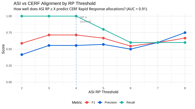
The plot below shows F1, precision, and recall for ASI at different RP thresholds against CERF Rapid Response allocations.

Code
p_asi_cerf <- df_rp_sensitivity |>
    select(rp_threshold, cerf_f1, cerf_precision, cerf_recall) |>
    pivot_longer(cols = c(cerf_f1, cerf_precision, cerf_recall),
                 names_to = "metric", values_to = "value") |>
    mutate(metric = case_when(
        metric == "cerf_f1" ~ "F1",
        metric == "cerf_precision" ~ "Precision",
        metric == "cerf_recall" ~ "Recall"
    )) |>
    ggplot(aes(x = rp_threshold, y = value, color = metric)) +
    geom_line(linewidth = 1) +
    geom_point(size = 3) +
    geom_vline(xintercept = 4, linetype = "dashed", alpha = 0.5) +
    annotate("text", x = 4.15, y = 0.95, label = "RP 4\n(current)", hjust = 0, size = 3) +
    scale_x_continuous(breaks = 2:8) +
    scale_y_continuous(limits = c(0, 1)) +
    scale_color_manual(values = c(
        "F1" = hdx_hex("tomato-hdx"),
        "Precision" = hdx_hex("sapphire-hdx"),
        "Recall" = hdx_hex("mint-hdx")
    )) +
    labs(
        title = "ASI vs CERF Alignment by RP Threshold",
        subtitle = glue("How well does ASI RP ≥ X predict CERF Rapid Response allocations? (AUC = {round(asi_auc, 2)})"),
        x = "ASI RP Threshold",
        y = "Score",
        color = "Metric"
    ) +
    theme_minimal() +
    theme(legend.position = "bottom")

ggsave("outputs/figures/fig-asi-cerf-alignment.png", p_asi_cerf, width = 8, height = 4.5, dpi = 300)

# Paper version with larger text
p_asi_cerf_paper <- p_asi_cerf + theme_minimal(base_size = 14) + theme(legend.position = "bottom")
ggsave("outputs/figures/paper/fig-asi-cerf-alignment.png", p_asi_cerf_paper, width = 8, height = 4.5, dpi = 300)

p_asi_cerf
Figure 13.1: ASI vs CERF Alignment by RP Threshold
Code
df_rp_sensitivity |>
    select(rp_threshold, n_drought_years, cerf_f1, cerf_precision, cerf_recall) |>
    gt() |>
    tab_header(
        title = "ASI-CERF Alignment by RP Threshold",
        subtitle = glue("Evaluating ASI RP ≥ X as predictor of CERF allocations (n = {nrow(df_asi_cerf)} years)")
    ) |>
    cols_label(
        rp_threshold = "RP Threshold",
        n_drought_years = "Years ≥ RP",
        cerf_f1 = "F1",
        cerf_precision = "Precision",
        cerf_recall = "Recall"
    ) |>
    fmt_number(columns = c(cerf_f1, cerf_precision, cerf_recall), decimals = 3) |>
    sub_missing(missing_text = "—") |>
    tab_style(
        style = cell_fill(color = "lightgreen"),
        locations = cells_body(rows = rp_threshold == 4)
    ) |>
    tab_footnote(
        footnote = "Green = current choice (RP ≥ 4)",
        locations = cells_column_labels(columns = rp_threshold)
    ) |>
    tab_footnote(
        footnote = "Count within CERF evaluation period (2006–2025) only; ASI RPs based on full 42-year climatology",
        locations = cells_column_labels(columns = n_drought_years)
    )
ASI-CERF Alignment by RP Threshold
Evaluating ASI RP ≥ X as predictor of CERF allocations (n = 20 years)
RP Threshold1 Years ≥ RP2 F1 Precision Recall
2 12 0.588 0.417 1.000
3 9 0.714 0.556 1.000
4 9 0.714 0.556 1.000
5 7 0.667 0.571 0.800
6 6 0.545 0.500 0.600
7 5 0.600 0.600 0.600
8 4 0.667 0.750 0.600
1 Green = current choice (RP ≥ 4)
2 Count within CERF evaluation period (2006–2025) only; ASI RPs based on full 42-year climatology

13.8.2 Which ASI years align with CERF?

Code
# Show ASI drought years vs CERF years
cerf_years <- df_cerf_yr |> filter(cerf == "yes") |> pull(yr)

df_asi_cerf |>
    mutate(
        asi_rp3 = if_else(asi_rp >= 3, "✓", ""),
        asi_rp4 = if_else(asi_rp >= 4, "✓", ""),
        asi_rp5 = if_else(asi_rp >= 5, "✓", ""),
        cerf = if_else(pub_year %in% cerf_years, "✓", "")
    ) |>
    select(pub_year, asi_rp3, asi_rp4, asi_rp5, cerf) |>
    arrange(desc(pub_year)) |>
    gt() |>
    tab_header(
        title = "ASI Drought Years vs CERF Allocations",
        subtitle = "Does ASI RP ≥ X capture CERF years?"
    ) |>
    cols_label(
        pub_year = "Year",
        asi_rp3 = "RP ≥ 3",
        asi_rp4 = "RP ≥ 4",
        asi_rp5 = "RP ≥ 5",
        cerf = "CERF"
    ) |>
    tab_style(
        style = cell_fill(color = "tomato", alpha = 0.3),
        locations = cells_body(columns = cerf, rows = cerf == "✓")
    ) |>
    tab_style(
        style = cell_fill(color = "lightgreen", alpha = 0.3),
        locations = cells_body(columns = asi_rp4)
    ) |>
    tab_spanner(label = "ASI Threshold", columns = c(asi_rp3, asi_rp4, asi_rp5))
Table 13.1: ASI Drought Years vs CERF Allocations
ASI Drought Years vs CERF Allocations
Does ASI RP ≥ X capture CERF years?
Year ASI Threshold CERF
RP ≥ 3 RP ≥ 4 RP ≥ 5
2025
2024
2023
2022
2021
2020
2019
2018
2017
2016
2015
2014
2013
2012
2011
2010
2009
2008
2007
2006
NoteASI Threshold Findings

Key observations:

  1. ASI-CERF relationship: ASI achieves AUC = 0.91 against CERF allocations, indicating the outcome variable does capture droughts that warranted humanitarian response
  2. Threshold sensitivity: The plot shows how precision/recall trade off as the RP threshold increases
  3. RP 4 rationale:
    • Captures ~9 years out of 20 (~45%)
    • Represents “worse than 1-in-4 years” — severe enough to warrant early action
    • Aligns with typical AA activation frequencies (every 3-5 years)