Appendix B — Multi-Year Drought Analysis

This chapter examines multi-year consecutive drought events using ERA5 MAM (March-April-May) precipitation data. We quantify the probability of consecutive drought years and develop return periods for multi-year drought events.

B.1 Key Questions

What is the probability of 2 or 3 consecutive drought years?
Is there persistence in drought years (i.e., if this year is drought, is next year more likely to be drought)?
What are the return periods for multi-year drought events?
How should we think about accumulated deficits over 2-3 year windows?

Code

library(tidyverse)
library(gghdx)
library(glue)
library(janitor)

gghdx()

box::use(
    cumulus
)

# Priority provinces (without Bamyan)
PROVINCES_AOI <- c(
    "Faryab",
    "Sar-e-Pul",
    "Badghis",
    "Takhar",
    "Badakhshan"
)

B.2 Load ERA5 MAM Precipitation Data

Load ERA5 precipitation directly from the database and join with polygon table to get province names.

Code

# Connect to database
con <- cumulus::pg_con()

# Get province names from polygon table
df_provinces <- tbl(con, "polygon") |>
    filter(iso3 == "AFG", adm_level == 1) |>
    select(pcode, name) |>
    distinct() |>
    collect() |>
    clean_names()

# Load ERA5 data for Afghanistan admin1
df_era5_raw <- tbl(con, "era5") |>
    filter(iso3 == "AFG", adm_level == 1) |>
    collect() |>
    clean_names() |>
    # Join with province names
    left_join(df_provinces, by = "pcode")

cat("=== ERA5 Data Loaded ===\n")

=== ERA5 Data Loaded ===

Code

cat("Date range:", as.character(min(df_era5_raw$valid_date)), "to",
    as.character(max(df_era5_raw$valid_date)), "\n")

Date range: 1981-01-01 to 2025-12-01

Code

cat("Provinces:", length(unique(df_era5_raw$pcode)), "\n")

Provinces: 34

Code

# Process to MAM totals per province per year
df_era5_mam <- df_era5_raw |>
    mutate(
        year = year(valid_date),
        month = month(valid_date)
    ) |>
    # Filter to MAM months
    filter(month %in% c(3, 4, 5)) |>
    # Use the 'mean' column (mean precipitation in mm)
    group_by(name, pcode, year) |>
    summarise(
        mam_precip = sum(mean, na.rm = TRUE),
        n_months = n(),
        .groups = "drop"
    ) |>
    # Only keep complete years (all 3 months)
    filter(n_months == 3) |>
    # Filter to priority provinces
    filter(name %in% PROVINCES_AOI) |>
    arrange(name, year)

# Summary
cat("\n=== ERA5 MAM Precipitation Summary ===\n")


=== ERA5 MAM Precipitation Summary ===

Code

cat("Years:", min(df_era5_mam$year), "-", max(df_era5_mam$year), "\n")

Years: 1981 - 2025

Code

cat("Provinces:", paste(unique(df_era5_mam$name), collapse = ", "), "\n")

Provinces: Badakhshan, Badghis, Faryab, Sar-e-Pul, Takhar

Code

cat("Records per province:\n")

Records per province:

Code

df_era5_mam |> count(name) |> print()

# A tibble: 5 × 2
  name           n
  <chr>      <int>
1 Badakhshan    45
2 Badghis       45
3 Faryab        45
4 Sar-e-Pul     45
5 Takhar        45

B.3 Define Drought Threshold

We define a “drought year” as MAM precipitation below the 5-year return period threshold (20th percentile) for each province.

Code

# Configuration
DROUGHT_RP <- 5  # 5-year return period = 20th percentile

# Calculate province-specific drought thresholds
df_thresholds <- df_era5_mam |>
    group_by(name) |>
    summarise(
        n_years = n(),
        mean_precip = mean(mam_precip),
        sd_precip = sd(mam_precip),
        # 20th percentile for 5-year RP drought
        threshold_5yr = quantile(mam_precip, probs = 1/DROUGHT_RP),
        threshold_3yr = quantile(mam_precip, probs = 1/3),
        .groups = "drop"
    )

cat("Drought Thresholds (", DROUGHT_RP, "-year RP):\n\n", sep = "")

Drought Thresholds (5-year RP):

Code

df_thresholds |>
    mutate(across(where(is.numeric), ~round(.x, 1))) |>
    print()

# A tibble: 5 × 6
  name       n_years mean_precip sd_precip threshold_5yr threshold_3yr
  <chr>        <dbl>       <dbl>     <dbl>         <dbl>         <dbl>
1 Badakhshan      45         8.8       1.7           7.5           8.1
2 Badghis         45         5.8       1.9           3.8           5  
3 Faryab          45         5.8       1.8           4.1           5.1
4 Sar-e-Pul       45         6.6       1.7           5.4           6.1
5 Takhar          45         9.6       2.3           8.1           8.9

Code

# Classify each year as drought or normal
df_drought_classified <- df_era5_mam |>
    left_join(df_thresholds |> select(name, threshold_5yr), by = "name") |>
    mutate(
        is_drought = mam_precip < threshold_5yr,
        drought_flag = as.integer(is_drought)
    )

# Summary by province
cat("\nDrought Years by Province:\n")


Drought Years by Province:

Code

df_drought_classified |>
    group_by(name) |>
    summarise(
        n_years = n(),
        n_drought = sum(is_drought),
        pct_drought = round(100 * mean(is_drought), 1),
        empirical_rp = round(n_years / n_drought, 1),
        .groups = "drop"
    ) |>
    print()

# A tibble: 5 × 5
  name       n_years n_drought pct_drought empirical_rp
  <chr>        <int>     <int>       <dbl>        <dbl>
1 Badakhshan      45         9          20            5
2 Badghis         45         9          20            5
3 Faryab          45         9          20            5
4 Sar-e-Pul       45         9          20            5
5 Takhar          45         9          20            5

B.4 Visualize Drought Years

Code

ggplot(df_drought_classified, aes(x = year, y = mam_precip)) +
    geom_col(aes(fill = is_drought), width = 0.8) +
    geom_hline(
        data = df_thresholds,
        aes(yintercept = threshold_5yr),
        linetype = "dashed", color = "red", linewidth = 0.8
    ) +
    facet_wrap(~name, scales = "free_y", ncol = 2) +
    scale_fill_manual(
        values = c("FALSE" = "#56B4E9", "TRUE" = "#D55E00"),
        labels = c("FALSE" = "Normal", "TRUE" = "Drought"),
        name = NULL
    ) +
    labs(
        title = "MAM Precipitation by Province with Drought Classification",
        subtitle = glue("Red dashed line = {DROUGHT_RP}-year RP drought threshold (20th percentile)"),
        x = "Year",
        y = "MAM Precipitation (mm)"
    ) +
    theme(legend.position = "bottom")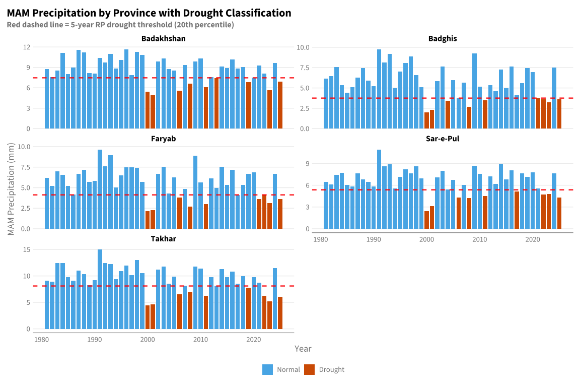

B.5 Multi-Year Drought Runs: Empirical Analysis

Count consecutive drought years in the historical record.

Code

# Function to identify runs of consecutive droughts
identify_runs <- function(drought_vector) {
    rle_result <- rle(drought_vector)

    # Get runs of TRUE (drought)
    drought_runs <- tibble(
        run_length = rle_result$lengths[rle_result$values == TRUE],
        is_drought = TRUE
    )

    if (nrow(drought_runs) == 0) {
        return(tibble(run_length = integer(), count = integer()))
    }

    drought_runs |>
        count(run_length) |>
        rename(count = n)
}

# Calculate runs for each province
df_runs_by_province <- df_drought_classified |>
    arrange(name, year) |>
    group_by(name) |>
    summarise(
        runs = list(identify_runs(is_drought)),
        .groups = "drop"
    ) |>
    unnest(runs)

cat("Drought Runs by Province:\n")

Drought Runs by Province:

Code

df_runs_by_province |>
    pivot_wider(names_from = run_length, values_from = count,
                names_prefix = "run_", values_fill = 0) |>
    print()

# A tibble: 5 × 4
  name       run_1 run_2 run_3
  <chr>      <int> <int> <int>
1 Badakhshan     7     1     0
2 Badghis        4     1     1
3 Faryab         4     1     1
4 Sar-e-Pul      5     2     0
5 Takhar         5     2     0

Code

# Aggregate across provinces
df_runs_total <- df_runs_by_province |>
    group_by(run_length) |>
    summarise(total_count = sum(count), .groups = "drop")

cat("\n\nTotal Drought Run Distribution (all provinces):\n")



Total Drought Run Distribution (all provinces):

Code

df_runs_total |>
    mutate(
        description = case_when(
            run_length == 1 ~ "Single drought year",
            run_length == 2 ~ "2 consecutive years",
            run_length == 3 ~ "3 consecutive years",
            TRUE ~ paste0(run_length, " consecutive years")
        )
    ) |>
    print()

# A tibble: 3 × 3
  run_length total_count description        
       <int>       <int> <chr>              
1          1          25 Single drought year
2          2           7 2 consecutive years
3          3           2 3 consecutive years

B.6 Markov Chain Analysis: Drought Persistence

Estimate transition probabilities to understand drought persistence.

Code

# Calculate transitions across all provinces (pooled)
df_transitions <- df_drought_classified |>
    arrange(name, year) |>
    group_by(name) |>
    mutate(prev_drought = lag(is_drought)) |>
    filter(!is.na(prev_drought)) |>
    ungroup()

# Count transitions
n_dd <- sum(df_transitions$prev_drought & df_transitions$is_drought)
n_dn <- sum(df_transitions$prev_drought & !df_transitions$is_drought)
n_nd <- sum(!df_transitions$prev_drought & df_transitions$is_drought)
n_nn <- sum(!df_transitions$prev_drought & !df_transitions$is_drought)

# Calculate probabilities
p_dd <- n_dd / (n_dd + n_dn)  # P(drought | previous drought)
p_nd <- n_nd / (n_nd + n_nn)  # P(drought | previous normal)

cat("=== Markov Transition Analysis (Pooled Across Provinces) ===\n\n")

=== Markov Transition Analysis (Pooled Across Provinces) ===

Code

cat("Transition Counts:\n")

Transition Counts:

Code

cat("  D → D:", n_dd, "\n")

  D → D: 11

Code

cat("  D → N:", n_dn, "\n")

  D → N: 29

Code

cat("  N → D:", n_nd, "\n")

  N → D: 34

Code

cat("  N → N:", n_nn, "\n\n")

  N → N: 146

Code

cat("Transition Probabilities:\n")

Transition Probabilities:

Code

cat("  P(Drought | Previous Drought) = p_dd =", round(p_dd, 3), "\n")

  P(Drought | Previous Drought) = p_dd = 0.275

Code

cat("  P(Drought | Previous Normal)  = p_nd =", round(p_nd, 3), "\n\n")

  P(Drought | Previous Normal)  = p_nd = 0.189

Code

cat("Persistence Analysis:\n")

Persistence Analysis:

Code

cat("  Persistence ratio (p_dd / p_nd) =", round(p_dd / p_nd, 2), "\n")

  Persistence ratio (p_dd / p_nd) = 1.46

Code

cat("  (Ratio > 1 indicates positive autocorrelation / drought persistence)\n")

  (Ratio > 1 indicates positive autocorrelation / drought persistence)

B.7 Lag-1 Autocorrelation

Code

# Calculate lag-1 autocorrelation for each province
df_autocorr <- df_drought_classified |>
    group_by(name) |>
    arrange(year) |>
    summarise(
        lag1_corr_precip = cor(mam_precip, lag(mam_precip), use = "complete.obs"),
        lag1_corr_drought = cor(drought_flag, lag(drought_flag), use = "complete.obs"),
        .groups = "drop"
    )

cat("Lag-1 Autocorrelation by Province:\n")

Lag-1 Autocorrelation by Province:

Code

df_autocorr |>
    mutate(across(where(is.numeric), ~round(.x, 3))) |>
    print()

# A tibble: 5 × 3
  name       lag1_corr_precip lag1_corr_drought
  <chr>                 <dbl>             <dbl>
1 Badakhshan            0.085            -0.093
2 Badghis               0.125             0.199
3 Faryab                0.112             0.199
4 Sar-e-Pul             0.127             0.053
5 Takhar                0.199             0.053

Code

# Visualize year-to-year persistence
df_drought_classified |>
    arrange(name, year) |>
    group_by(name) |>
    mutate(prev_precip = lag(mam_precip)) |>
    filter(!is.na(prev_precip)) |>
    ggplot(aes(x = prev_precip, y = mam_precip)) +
    geom_point(aes(color = is_drought), alpha = 0.7, size = 2) +
    geom_smooth(method = "lm", se = TRUE, color = "black", linetype = "dashed") +
    facet_wrap(~name, scales = "free") +
    scale_color_manual(
        values = c("FALSE" = "#56B4E9", "TRUE" = "#D55E00"),
        labels = c("FALSE" = "Normal", "TRUE" = "Drought")
    ) +
    labs(
        title = "Year-to-Year Precipitation Persistence",
        subtitle = "Dashed line = linear fit showing lag-1 autocorrelation",
        x = "Previous Year MAM Precipitation (mm)",
        y = "Current Year MAM Precipitation (mm)",
        color = "Current Year"
    ) +
    theme(legend.position = "bottom")

`geom_smooth()` using formula = 'y ~ x'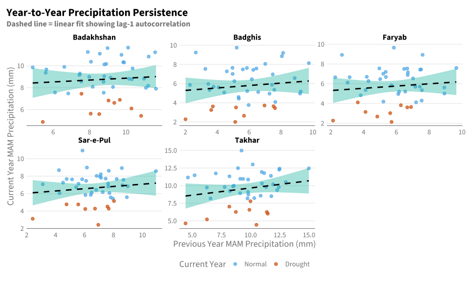

B.8 Multi-Year Drought Probabilities: Markov Model

Using the estimated transition probabilities, calculate theoretical probabilities of consecutive drought years.

Code

# Stationary probability of drought
# pi_D = p_nd / (p_nd + (1 - p_dd))
pi_D <- p_nd / (p_nd + (1 - p_dd))

# Probability of n consecutive drought years
# P(run of n starting from drought) = pi_D * p_dd^(n-1)
calc_consecutive_prob <- function(n, pi_D, p_dd) {
    pi_D * p_dd^(n-1)
}

# Under independence assumption for comparison
p_drought_independent <- mean(df_drought_classified$is_drought)

# Build comparison table
df_multiyear_prob <- tibble(
    consecutive_years = 1:5
) |>
    mutate(
        # Markov model (accounts for persistence)
        prob_markov = map_dbl(consecutive_years, ~calc_consecutive_prob(.x, pi_D, p_dd)),
        rp_markov = 1 / prob_markov,

        # Independence assumption (no persistence)
        prob_independent = p_drought_independent^consecutive_years,
        rp_independent = 1 / prob_independent
    )

cat("=== Multi-Year Drought Probabilities ===\n\n")

=== Multi-Year Drought Probabilities ===

Code

cat("Stationary P(Drought) =", round(pi_D, 3), "\n")

Stationary P(Drought) = 0.207

Code

cat("Persistence P(D|D) =", round(p_dd, 3), "\n")

Persistence P(D|D) = 0.275

Code

cat("Marginal P(Drought) =", round(p_drought_independent, 3), "\n\n")

Marginal P(Drought) = 0.2

Code

df_multiyear_prob |>
    mutate(
        `P (Markov)` = paste0(round(prob_markov * 100, 2), "%"),
        `RP (Markov)` = paste0(round(rp_markov, 1), " yr"),
        `P (Independent)` = paste0(round(prob_independent * 100, 2), "%"),
        `RP (Independent)` = paste0(round(rp_independent, 1), " yr")
    ) |>
    select(consecutive_years, `P (Markov)`, `RP (Markov)`, `P (Independent)`, `RP (Independent)`) |>
    print()

# A tibble: 5 × 5
  consecutive_years `P (Markov)` `RP (Markov)` `P (Independent)`
              <int> <chr>        <chr>         <chr>            
1                 1 20.67%       4.8 yr        20%              
2                 2 5.68%        17.6 yr       4%               
3                 3 1.56%        64 yr         0.8%             
4                 4 0.43%        232.6 yr      0.16%            
5                 5 0.12%        846 yr        0.03%            
# ℹ 1 more variable: `RP (Independent)` <chr>

Code

df_plot_probs <- df_multiyear_prob |>
    select(consecutive_years, prob_markov, prob_independent) |>
    pivot_longer(
        cols = c(prob_markov, prob_independent),
        names_to = "model",
        values_to = "probability"
    ) |>
    mutate(
        model = case_when(
            model == "prob_markov" ~ "Markov (with persistence)",
            model == "prob_independent" ~ "Independence (no persistence)"
        )
    )

ggplot(df_plot_probs, aes(x = factor(consecutive_years), y = probability * 100, fill = model)) +
    geom_col(position = position_dodge(width = 0.8), width = 0.7) +
    geom_text(
        aes(label = paste0(round(probability * 100, 1), "%")),
        position = position_dodge(width = 0.8),
        vjust = -0.5, size = 3.5
    ) +
    scale_fill_manual(values = c("Markov (with persistence)" = "#E69F00",
                                  "Independence (no persistence)" = "#56B4E9")) +
    scale_y_continuous(limits = c(0, max(df_plot_probs$probability) * 100 * 1.3)) +
    labs(
        title = "Probability of Consecutive Drought Years",
        subtitle = glue("Drought defined as MAM precipitation below {DROUGHT_RP}-year RP threshold"),
        x = "Number of Consecutive Drought Years",
        y = "Probability (%)",
        fill = NULL
    ) +
    theme(legend.position = "bottom")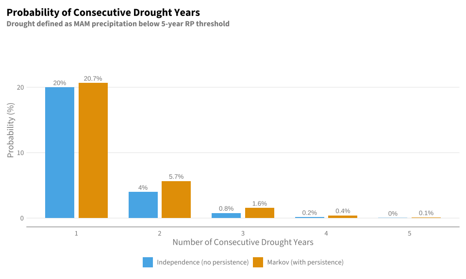

B.9 Accumulated Deficit Analysis

Instead of just counting consecutive drought years, we can examine the accumulated precipitation deficit over 2-3 year windows.

Code

# Calculate rolling 2-year and 3-year MAM precipitation totals
df_accumulated <- df_era5_mam |>
    arrange(name, year) |>
    group_by(name) |>
    mutate(
        precip_2yr = zoo::rollsum(mam_precip, k = 2, fill = NA, align = "right"),
        precip_3yr = zoo::rollsum(mam_precip, k = 3, fill = NA, align = "right")
    ) |>
    ungroup()

# Calculate thresholds for accumulated deficits
df_accum_thresholds <- df_accumulated |>
    group_by(name) |>
    summarise(
        # Climatological means
        mean_2yr = mean(precip_2yr, na.rm = TRUE),
        mean_3yr = mean(precip_3yr, na.rm = TRUE),
        # 5-year RP thresholds (20th percentile)
        threshold_2yr_5rp = quantile(precip_2yr, probs = 0.2, na.rm = TRUE),
        threshold_3yr_5rp = quantile(precip_3yr, probs = 0.2, na.rm = TRUE),
        .groups = "drop"
    )

cat("Accumulated Precipitation Thresholds (5-year RP):\n")

Accumulated Precipitation Thresholds (5-year RP):

Code

df_accum_thresholds |>
    mutate(across(where(is.numeric), ~round(.x, 1))) |>
    print()

# A tibble: 5 × 5
  name       mean_2yr mean_3yr threshold_2yr_5rp threshold_3yr_5rp
  <chr>         <dbl>    <dbl>             <dbl>             <dbl>
1 Badakhshan     17.6     26.4              15.6              23.4
2 Badghis        11.6     17.4               9.4              14.3
3 Faryab         11.6     17.3               9.3              14.7
4 Sar-e-Pul      13.4     20.1              11.9              18  
5 Takhar         19.3     28.9              16.6              24.9

Code

# Plot 2-year accumulated precipitation
df_accumulated |>
    filter(!is.na(precip_2yr)) |>
    left_join(
        df_accum_thresholds |> select(name, threshold_2yr_5rp, mean_2yr),
        by = "name"
    ) |>
    mutate(below_threshold = precip_2yr < threshold_2yr_5rp) |>
    ggplot(aes(x = year, y = precip_2yr)) +
    geom_col(aes(fill = below_threshold), width = 0.8) +
    geom_hline(aes(yintercept = threshold_2yr_5rp), linetype = "dashed", color = "red") +
    geom_hline(aes(yintercept = mean_2yr), linetype = "solid", color = "gray40", alpha = 0.7) +
    facet_wrap(~name, scales = "free_y", ncol = 2) +
    scale_fill_manual(
        values = c("FALSE" = "#56B4E9", "TRUE" = "#D55E00"),
        labels = c("FALSE" = "Normal", "TRUE" = "Deficit")
    ) +
    labs(
        title = "2-Year Accumulated MAM Precipitation",
        subtitle = "Red dashed = 5-year RP threshold | Gray solid = climatological mean",
        x = "Year (end of 2-year window)",
        y = "2-Year Accumulated Precipitation (mm)",
        fill = NULL
    ) +
    theme(legend.position = "bottom")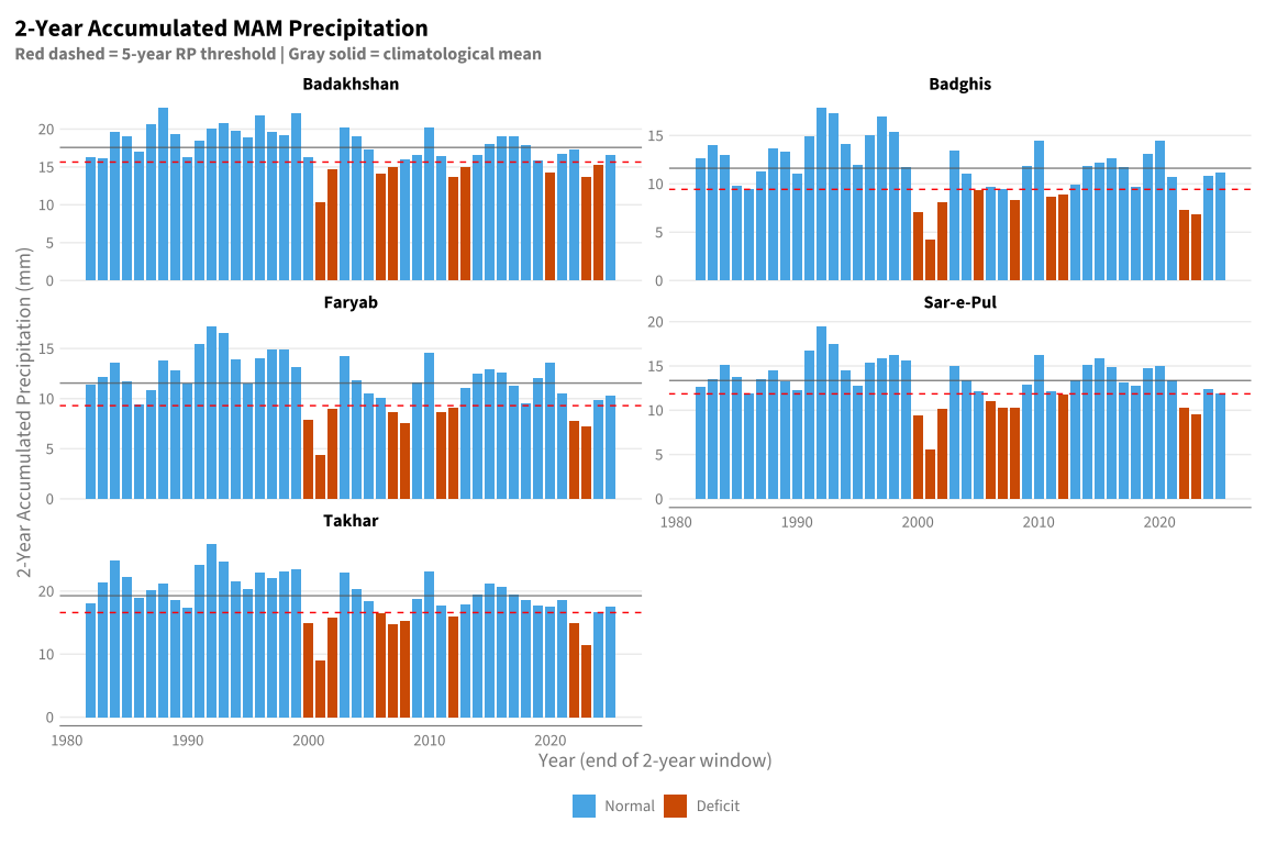

B.10 Summary: Multi-Year Drought Framework

Code

cat("=" |> rep(60) |> paste(collapse = ""), "\n")

============================================================

Code

cat("MULTI-YEAR DROUGHT ANALYSIS SUMMARY\n")

MULTI-YEAR DROUGHT ANALYSIS SUMMARY

Code

cat("=" |> rep(60) |> paste(collapse = ""), "\n\n")

============================================================

Code

cat("DATA:\n")

DATA:

Code

cat("  - ERA5 MAM (Mar-Apr-May) precipitation, ", min(df_era5_mam$year), "-", max(df_era5_mam$year), "\n", sep = "")

  - ERA5 MAM (Mar-Apr-May) precipitation, 1981-2025

Code

cat("  - ", length(unique(df_era5_mam$name)), " priority provinces\n\n", sep = "")

  - 5 priority provinces

Code

cat("DROUGHT DEFINITION:\n")

DROUGHT DEFINITION:

Code

cat("  - Single year: MAM precip below ", DROUGHT_RP, "-year RP threshold (20th percentile)\n\n", sep = "")

  - Single year: MAM precip below 5-year RP threshold (20th percentile)

Code

cat("PERSISTENCE (Markov Model):\n")

PERSISTENCE (Markov Model):

Code

cat("  - P(Drought | Previous Drought) = ", round(p_dd * 100, 1), "%\n", sep = "")

  - P(Drought | Previous Drought) = 27.5%

Code

cat("  - P(Drought | Previous Normal)  = ", round(p_nd * 100, 1), "%\n", sep = "")

  - P(Drought | Previous Normal)  = 18.9%

Code

cat("  - Persistence ratio = ", round(p_dd / p_nd, 2), " (>1 = positive autocorrelation)\n\n", sep = "")

  - Persistence ratio = 1.46 (>1 = positive autocorrelation)

Code

cat("MULTI-YEAR DROUGHT PROBABILITIES (Markov Model):\n")

MULTI-YEAR DROUGHT PROBABILITIES (Markov Model):

Code

for (i in 1:3) {
    prob <- calc_consecutive_prob(i, pi_D, p_dd)
    cat("  - ", i, " consecutive year(s): ", round(prob * 100, 2),
        "% (RP = ", round(1/prob, 1), " years)\n", sep = "")
}

  - 1 consecutive year(s): 20.67% (RP = 4.8 years)
  - 2 consecutive year(s): 5.68% (RP = 17.6 years)
  - 3 consecutive year(s): 1.56% (RP = 64 years)

Code

cat("\nKEY INSIGHT:\n")


KEY INSIGHT:

Code

if (p_dd > p_nd) {
    cat("  Drought years show POSITIVE persistence (p_dd > p_nd).\n")
    cat("  Multi-year droughts are MORE likely than independence would suggest.\n")
} else {
    cat("  No significant drought persistence detected.\n")
}

  Drought years show POSITIVE persistence (p_dd > p_nd).
  Multi-year droughts are MORE likely than independence would suggest.

B.11 Application: Conditional Probability Tool

Given a new MAM rainfall observation, what’s the probability of multi-year drought?

Code

# Function to assess multi-year drought risk given current year status
assess_multiyear_risk <- function(current_year_drought, p_dd, p_nd) {
    if (current_year_drought) {
        cat("Current year: DROUGHT\n")
        cat("  P(Next year drought) = ", round(p_dd * 100, 1), "%\n", sep = "")
        cat("  P(2 consecutive from here) = ", round(p_dd * 100, 1), "%\n", sep = "")
        cat("  P(3 consecutive from here) = ", round(p_dd^2 * 100, 1), "%\n", sep = "")
    } else {
        cat("Current year: NORMAL\n")
        cat("  P(Next year drought) = ", round(p_nd * 100, 1), "%\n", sep = "")
        cat("  P(2 consecutive starting next year) = ", round(p_nd * p_dd * 100, 2), "%\n", sep = "")
    }
}

cat("SCENARIO 1: Current year is a DROUGHT year\n")

SCENARIO 1: Current year is a DROUGHT year

Code

cat("-" |> rep(40) |> paste(collapse = ""), "\n")

----------------------------------------

Code

assess_multiyear_risk(TRUE, p_dd, p_nd)

Current year: DROUGHT
  P(Next year drought) = 27.5%
  P(2 consecutive from here) = 27.5%
  P(3 consecutive from here) = 7.6%

Code

cat("\n\nSCENARIO 2: Current year is NORMAL\n")



SCENARIO 2: Current year is NORMAL

Code

cat("-" |> rep(40) |> paste(collapse = ""), "\n")

----------------------------------------

Code

assess_multiyear_risk(FALSE, p_dd, p_nd)

Current year: NORMAL
  P(Next year drought) = 18.9%
  P(2 consecutive starting next year) = 5.19%

B.12 Probability of 2 Consecutive Drought Years (Any Given Year)

Given any arbitrary year, what is the probability that it begins a 2-year consecutive drought?

\[P(\text{2 consecutive droughts starting year } t) = P(D_t) \times P(D_{t+1} | D_t) = \pi_D \times p_{dd}\]

Code

# P(this year AND next year are both droughts)
p_2yr_consecutive <- pi_D * p_dd
rp_2yr_consecutive <- 1 / p_2yr_consecutive

cat("=== Probability of 2 Consecutive Drought Years (from any given year) ===\n\n")

=== Probability of 2 Consecutive Drought Years (from any given year) ===

Code

cat("P(Year t is drought) = π_D = ", round(pi_D * 100, 2), "%\n", sep = "")

P(Year t is drought) = π_D = 20.67%

Code

cat("P(Year t+1 is drought | Year t is drought) = p_dd = ", round(p_dd * 100, 2), "%\n\n", sep = "")

P(Year t+1 is drought | Year t is drought) = p_dd = 27.5%

Code

cat("P(2 consecutive droughts starting any year) = π_D × p_dd\n")

P(2 consecutive droughts starting any year) = π_D × p_dd

Code

cat("                                            = ", round(p_2yr_consecutive * 100, 2), "%\n\n", sep = "")

                                            = 5.68%

Code

cat("RETURN PERIOD: ", round(rp_2yr_consecutive, 1), " years\n", sep = "")

RETURN PERIOD: 17.6 years

B.13 Finding Single-Year Thresholds for Target 2-Consecutive RPs

What single-year drought threshold (RP) would give us a specific 2-consecutive-year return period?

B.13.1 Theoretical Approach (Independence Assumption)

Under independence: \(P(\text{2 consecutive}) = p^2\) where \(p = 1/\text{RP}_{\text{single}}\)

Therefore: \(\text{RP}_{\text{single}} = \sqrt{\text{RP}_{\text{2-consecutive}}}\)

Code

target_2yr_rps <- c(3, 4, 5, 6, 7, 8)

df_theoretical <- tibble(
    target_2yr_rp = target_2yr_rps,
    single_yr_rp_independent = sqrt(target_2yr_rps),
    single_yr_prob_independent = 1 / single_yr_rp_independent
)

cat("Theoretical Single-Year Thresholds (Independence Assumption):\n\n")

Theoretical Single-Year Thresholds (Independence Assumption):

Code

df_theoretical |>
    mutate(
        `Target 2-Consec RP` = paste0(target_2yr_rp, " yr"),
        `Single-Year RP` = round(single_yr_rp_independent, 2),
        `Single-Year Prob` = paste0(round(single_yr_prob_independent * 100, 1), "%"),
        `Percentile Threshold` = paste0(round(single_yr_prob_independent * 100, 1), "th")
    ) |>
    select(`Target 2-Consec RP`, `Single-Year RP`, `Single-Year Prob`, `Percentile Threshold`) |>
    print()

# A tibble: 6 × 4
  `Target 2-Consec RP` `Single-Year RP` `Single-Year Prob`
  <chr>                           <dbl> <chr>             
1 3 yr                             1.73 57.7%             
2 4 yr                             2    50%               
3 5 yr                             2.24 44.7%             
4 6 yr                             2.45 40.8%             
5 7 yr                             2.65 37.8%             
6 8 yr                             2.83 35.4%             
# ℹ 1 more variable: `Percentile Threshold` <chr>

B.13.2 Empirical Approach (Accounting for Persistence)

Sweep through different single-year thresholds and calculate the actual 2-consecutive RP accounting for Markov persistence.

Code

# Function to calculate 2-consecutive RP for a given single-year RP threshold
calc_2yr_rp_for_threshold <- function(data, single_yr_rp) {
    # Calculate threshold as percentile
    threshold_prob <- 1 / single_yr_rp

    # Apply threshold per province
    df_classified <- data |>
        group_by(name) |>
        mutate(
            threshold = quantile(mam_precip, probs = threshold_prob),
            is_drought = mam_precip < threshold
        ) |>
        ungroup()

    # Calculate Markov transitions
    df_trans <- df_classified |>
        arrange(name, year) |>
        group_by(name) |>
        mutate(prev_drought = lag(is_drought)) |>
        filter(!is.na(prev_drought)) |>
        ungroup()

    n_dd <- sum(df_trans$prev_drought & df_trans$is_drought)
    n_dn <- sum(df_trans$prev_drought & !df_trans$is_drought)
    n_nd <- sum(!df_trans$prev_drought & df_trans$is_drought)
    n_nn <- sum(!df_trans$prev_drought & !df_trans$is_drought)

    # Handle edge cases
    if ((n_dd + n_dn) == 0 || (n_nd + n_nn) == 0) {
        return(list(p_2yr = NA, rp_2yr = NA, p_dd = NA, p_nd = NA, pi_D = NA))
    }

    p_dd <- n_dd / (n_dd + n_dn)
    p_nd <- n_nd / (n_nd + n_nn)

    # Stationary probability
    pi_D <- p_nd / (p_nd + (1 - p_dd))

    # 2-consecutive probability
    p_2yr <- pi_D * p_dd
    rp_2yr <- 1 / p_2yr

    list(
        p_2yr = p_2yr,
        rp_2yr = rp_2yr,
        p_dd = p_dd,
        p_nd = p_nd,
        pi_D = pi_D
    )
}

# Sweep through single-year RPs from 1.5 to 10
single_yr_rps_sweep <- seq(1.5, 10, by = 0.25)

df_sweep <- tibble(single_yr_rp = single_yr_rps_sweep) |>
    mutate(
        results = map(single_yr_rp, ~calc_2yr_rp_for_threshold(df_era5_mam, .x))
    ) |>
    unnest_wider(results)

cat("Empirical Relationship: Single-Year RP → 2-Consecutive RP\n\n")

Empirical Relationship: Single-Year RP → 2-Consecutive RP

Code

df_sweep |>
    filter(!is.na(rp_2yr)) |>
    mutate(across(where(is.numeric), ~round(.x, 2))) |>
    select(single_yr_rp, pi_D, p_dd, rp_2yr) |>
    filter(single_yr_rp %in% c(2, 2.5, 3, 4, 5, 6, 8, 10)) |>
    print()

# A tibble: 8 × 4
  single_yr_rp  pi_D  p_dd rp_2yr
         <dbl> <dbl> <dbl>  <dbl>
1          2    0.49  0.48   4.32
2          2.5  0.4   0.36   6.8 
3          3    0.34  0.33   8.94
4          4    0.25  0.3   13.2 
5          5    0.21  0.28  17.6 
6          6    0.18  0.23  23.9 
7          8    0.14  0.22  32.6 
8         10    0.11  0.22  40.1

Code

# Interpolate to find single-year RPs for target 2-consecutive RPs
find_single_rp_for_target <- function(target_2yr_rp, sweep_data) {
    # Linear interpolation
    sweep_clean <- sweep_data |> filter(!is.na(rp_2yr))
    approx(x = sweep_clean$rp_2yr, y = sweep_clean$single_yr_rp, xout = target_2yr_rp)$y
}

df_target_thresholds <- tibble(
    target_2yr_rp = target_2yr_rps
) |>
    mutate(
        single_yr_rp_empirical = map_dbl(target_2yr_rp, ~find_single_rp_for_target(.x, df_sweep)),
        single_yr_rp_independent = sqrt(target_2yr_rp),
        percentile_empirical = 1 / single_yr_rp_empirical,
        percentile_independent = 1 / single_yr_rp_independent
    )

Warning: There were 6 warnings in `mutate()`.
The first warning was:
ℹ In argument: `single_yr_rp_empirical = map_dbl(target_2yr_rp,
  ~find_single_rp_for_target(.x, df_sweep))`.
Caused by warning in `regularize.values()`:
! collapsing to unique 'x' values
ℹ Run `dplyr::last_dplyr_warnings()` to see the 5 remaining warnings.

Code

cat("\n=== Single-Year Thresholds for Target 2-Consecutive RPs ===\n\n")


=== Single-Year Thresholds for Target 2-Consecutive RPs ===

Code

df_target_thresholds |>
    mutate(
        `Target 2-Yr RP` = paste0(target_2yr_rp, " yr"),
        `Single RP (Empirical)` = round(single_yr_rp_empirical, 2),
        `Single RP (Independent)` = round(single_yr_rp_independent, 2),
        `Percentile (Empirical)` = paste0(round(percentile_empirical * 100, 1), "%")
    ) |>
    select(`Target 2-Yr RP`, `Single RP (Empirical)`, `Single RP (Independent)`, `Percentile (Empirical)`) |>
    print()

# A tibble: 6 × 4
  `Target 2-Yr RP` `Single RP (Empirical)` `Single RP (Independent)`
  <chr>                              <dbl>                     <dbl>
1 3 yr                                1.76                      1.73
2 4 yr                                1.94                      2   
3 5 yr                                2.17                      2.24
4 6 yr                                2.36                      2.45
5 7 yr                                2.53                      2.65
6 8 yr                                2.7                       2.83
# ℹ 1 more variable: `Percentile (Empirical)` <chr>

Code

# Plot the relationship
ggplot(df_sweep |> filter(!is.na(rp_2yr), rp_2yr < 50), aes(x = single_yr_rp, y = rp_2yr)) +
    geom_line(linewidth = 1.2, color = "#E69F00") +
    geom_point(
        data = df_target_thresholds,
        aes(x = single_yr_rp_empirical, y = target_2yr_rp),
        size = 4, color = "#D55E00"
    ) +
    geom_text(
        data = df_target_thresholds,
        aes(x = single_yr_rp_empirical, y = target_2yr_rp,
            label = paste0(target_2yr_rp, "-yr")),
        vjust = -1, size = 3.5
    ) +
    geom_abline(
        aes(intercept = 0, slope = 1, linetype = "x² (independence)"),
        color = "gray50"
    ) +
    scale_linetype_manual(values = "dashed", name = NULL) +
    labs(
        title = "Single-Year RP Required for Target 2-Consecutive Drought RP",
        subtitle = "Orange line = empirical (with persistence) | Gray dashed = theoretical independence",
        x = "Single-Year Drought RP Threshold",
        y = "Resulting 2-Consecutive Drought RP"
    ) +
    theme(legend.position = "bottom")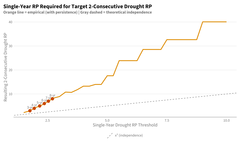

Code

cat("\n" , rep("=", 70) |> paste(collapse = ""), "\n", sep = "")


======================================================================

Code

cat("RECOMMENDED SINGLE-YEAR THRESHOLDS FOR 2-CONSECUTIVE DROUGHT RPs\n")

RECOMMENDED SINGLE-YEAR THRESHOLDS FOR 2-CONSECUTIVE DROUGHT RPs

Code

cat(rep("=", 70) |> paste(collapse = ""), "\n\n", sep = "")

======================================================================

Code

df_target_thresholds |>
    mutate(
        threshold_mm = map_dbl(single_yr_rp_empirical, function(rp) {
            # Get average threshold across provinces
            df_era5_mam |>
                group_by(name) |>
                summarise(thresh = quantile(mam_precip, probs = 1/rp), .groups = "drop") |>
                pull(thresh) |>
                mean()
        })
    ) |>
    transmute(
        `2-Consecutive RP` = paste0(target_2yr_rp, " years"),
        `Single-Year RP` = paste0(round(single_yr_rp_empirical, 2), " years"),
        `Percentile` = paste0(round(percentile_empirical * 100, 1), "%"),
        `Avg Threshold (mm)` = round(threshold_mm, 1)
    ) |>
    print()

# A tibble: 6 × 4
  `2-Consecutive RP` `Single-Year RP` Percentile `Avg Threshold (mm)`
  <chr>              <chr>            <chr>                     <dbl>
1 3 years            1.76 years       56.8%                       7.7
2 4 years            1.94 years       51.5%                       7.5
3 5 years            2.17 years       46.1%                       7.3
4 6 years            2.36 years       42.3%                       7.1
5 7 years            2.53 years       39.5%                       6.9
6 8 years            2.7 years        37%                         6.8